
使用 BART 建模异方差性#
在本笔记本中,我们将展示如何使用 BART 建模异方差性,如 pymc-bart 论文的第 4.1 节 [] 中所述。我们使用 R 包 datarium [] 提供的 marketing 数据集。我们的想法是将营销渠道对销售额的贡献建模为预算的函数。
import os

import arviz as az
import matplotlib.pyplot as plt
import numpy as np
import pandas as pd
import pymc as pm
import pymc_bart as pmb
%config InlineBackend.figure_format = "retina"
az.style.use("arviz-darkgrid")
plt.rcParams["figure.figsize"] = [10, 6]
rng = np.random.default_rng(42)
读取数据#
try:
    df = pd.read_csv(os.path.join("..", "data", "marketing.csv"), sep=";", decimal=",")
except FileNotFoundError:
    df = pd.read_csv(pm.get_data("marketing.csv"), sep=";", decimal=",")

n_obs = df.shape[0]

df.head()
| youtube | newspaper | sales | ||
|---|---|---|---|---|
| 0 | 276.12 | 45.36 | 83.04 | 26.52 |
| 1 | 53.40 | 47.16 | 54.12 | 12.48 |
| 2 | 20.64 | 55.08 | 83.16 | 11.16 |
| 3 | 181.80 | 49.56 | 70.20 | 22.20 |
| 4 | 216.96 | 12.96 | 70.08 | 15.48 |
EDA#
我们首先查看数据。我们将重点关注Youtube。
fig, ax = plt.subplots()
ax.plot(df["youtube"], df["sales"], "o", c="C0")
ax.set(title="Sales as a function of Youtube budget", xlabel="budget", ylabel="sales");
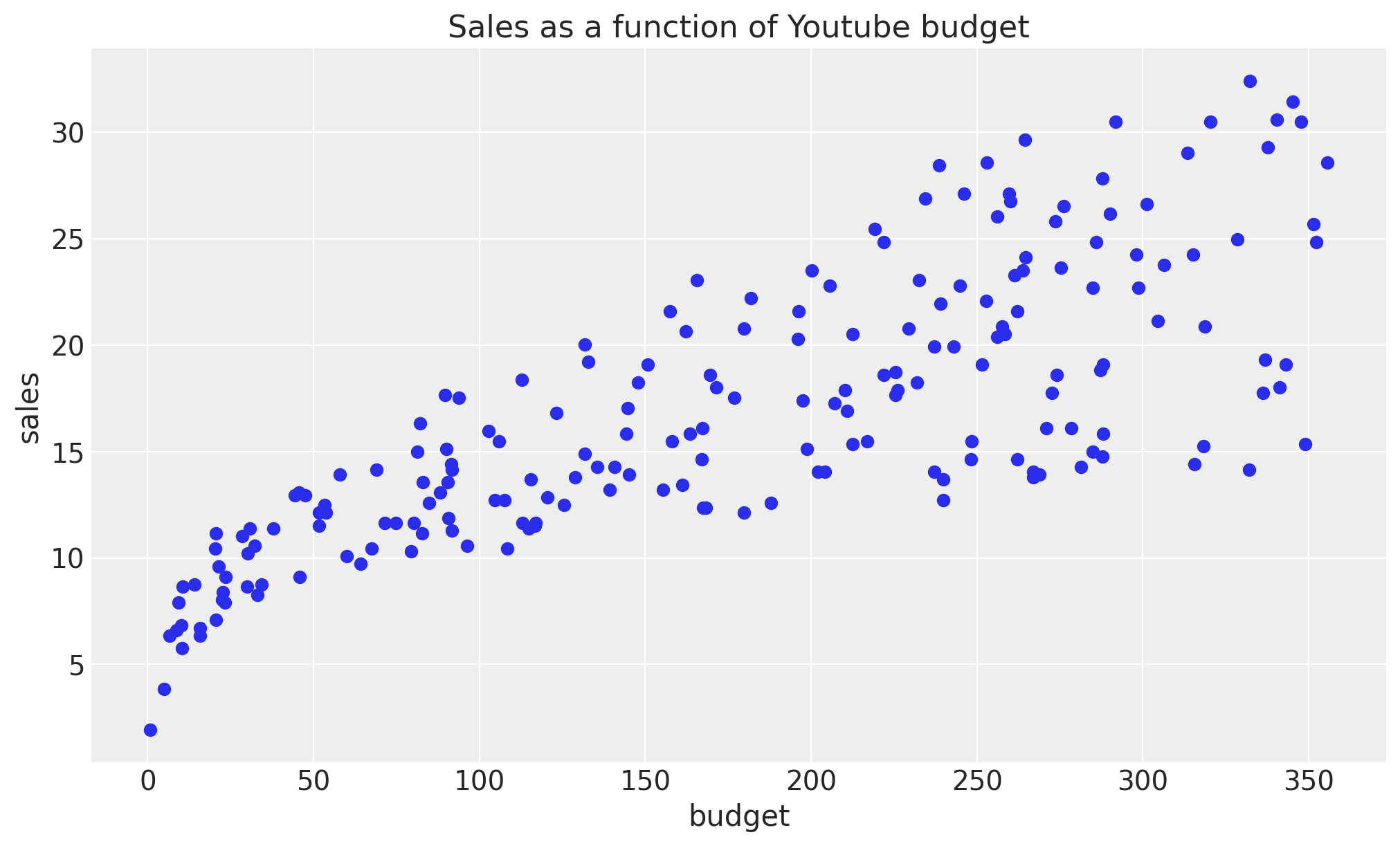
我们清楚地看到,均值和方差都随着预算的增加而增加。一种可能性是手动选择这些函数的显式参数化,例如平方根或对数。然而,在本例中,我们希望使用 BART 模型从数据中学习这些函数。
模型规范#
我们继续准备用于建模的数据。我们将使用 budget 作为预测变量,sales 作为响应变量。
X = df["youtube"].to_numpy().reshape(-1, 1)
Y = df["sales"].to_numpy()
接下来,我们指定模型。请注意,我们只需要一个 BART 分布,它可以向量化以同时建模均值和方差。我们使用 Gamma 分布作为似然函数,因为我们期望销售额为正。
with pm.Model() as model_marketing_full:
    w = pmb.BART("w", X=X, Y=np.log(Y), m=100, shape=(2, n_obs))
    y = pm.Gamma("y", mu=pm.math.exp(w[0]), sigma=pm.math.exp(w[1]), observed=Y)

pm.model_to_graphviz(model=model_marketing_full)

我们现在拟合模型。
with model_marketing_full:
    idata_marketing_full = pm.sample(2000, random_seed=rng, compute_convergence_checks=False)
    posterior_predictive_marketing_full = pm.sample_posterior_predictive(
        trace=idata_marketing_full, random_seed=rng
    )
Multiprocess sampling (4 chains in 4 jobs)
PGBART: [w]
Sampling 4 chains for 1_000 tune and 2_000 draw iterations (4_000 + 8_000 draws total) took 156 seconds.
Sampling: [y]
结果#
我们现在可以可视化均值和似然函数的后验预测分布。
posterior_mean = idata_marketing_full.posterior["w"].mean(dim=("chain", "draw"))[0]

w_hdi = az.hdi(ary=idata_marketing_full, group="posterior", var_names=["w"], hdi_prob=0.5)

pps = az.extract(
    posterior_predictive_marketing_full, group="posterior_predictive", var_names=["y"]
).T
idx = np.argsort(X[:, 0])


fig, ax = plt.subplots()
az.plot_hdi(
    x=X[:, 0],
    y=pps,
    ax=ax,
    hdi_prob=0.90,
    fill_kwargs={"alpha": 0.3, "label": r"Observations $90\%$ HDI"},
)
az.plot_hdi(
    x=X[:, 0],
    hdi_data=np.exp(w_hdi["w"].sel(w_dim_0=0)),
    ax=ax,
    fill_kwargs={"alpha": 0.6, "label": r"Mean $50\%$ HDI"},
)
ax.plot(df["youtube"], df["sales"], "o", c="C0", label="Raw Data")
ax.legend(loc="upper left")
ax.set(
    title="Sales as a function of Youtube budget - Posterior Predictive",
    xlabel="budget",
    ylabel="sales",
);
/home/osvaldo/proyectos/00_BM/arviz-devs/arviz/arviz/plots/hdiplot.py:161: FutureWarning: hdi currently interprets 2d data as (draw, shape) but this will change in a future release to (chain, draw) for coherence with other functions
  hdi_data = hdi(y, hdi_prob=hdi_prob, circular=circular, multimodal=False, **hdi_kwargs)
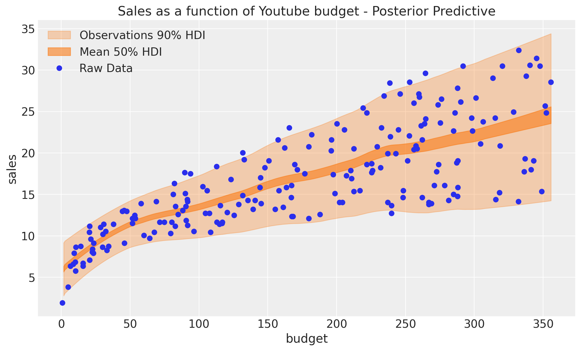
拟合效果看起来不错!事实上,我们看到均值和方差都随着预算的增加而增加。
参考文献#
水印#
%load_ext watermark
%watermark -n -u -v -iv -w -p pytensor
Last updated: Mon Dec 23 2024

Python implementation: CPython
Python version       : 3.11.5
IPython version      : 8.16.1

pytensor: 2.26.4

pymc_bart : 0.6.0
arviz     : 0.20.0.dev0
pymc      : 5.19.1
matplotlib: 3.8.4
pandas    : 2.1.2
numpy     : 1.26.4

Watermark: 2.4.3