先验和后验预测检查#

后验预测检查 (PPCs) 是验证模型的好方法。其理念是使用从后验分布中抽取的参数，从模型中生成数据。

稍微详细地说，可以说 PPCs 分析了从模型生成的数据偏离从真实分布生成的数据的程度。因此，通常您会想知道，例如，您的后验分布是否正在逼近您的底层分布。这种模型评估方法的可视化方面也非常适合进行‘理性检查’，或向他人解释您的模型并获得批评。

先验预测检查也是贝叶斯建模工作流程的关键部分。基本上，它们有两个主要好处

它们允许您检查您是否确实将科学知识融入到您的模型中——简而言之，它们帮助您检查在看到数据之前您的假设有多可信。
它们可以极大地帮助抽样，特别是对于广义线性模型，其中结果空间和参数空间由于链接函数而发散。

在这里，我们将实现一个通用例程，用于从模型的观察节点中抽取样本。这些模型是基本的，但它们将是创建您自己例程的垫脚石。如果您想了解如何在更复杂的多维模型中进行先验和后验预测检查，您可以查看这个 notebook。现在，让我们抽样！

import arviz as az
import matplotlib.pyplot as plt
import numpy as np
import xarray as xr

from scipy.special import expit as logistic

import pymc as pm

print(f"Running on PyMC v{pm.__version__}")

Running on PyMC v5.15.1+68.gc0b060b98.dirty

az.style.use("arviz-darkgrid")

RANDOM_SEED = 58
rng = np.random.default_rng(RANDOM_SEED)


def standardize(series):
    """Standardize a pandas series"""
    return (series - series.mean()) / series.std()

让我们生成一个非常简单的线性回归模型。为了特意说明，我将模拟不来自标准正态分布的数据（稍后您会明白为什么）

N = 100

true_a, true_b, predictor = 0.5, 3.0, rng.normal(loc=2, scale=6, size=N)
true_mu = true_a + true_b * predictor
true_sd = 2.0

outcome = rng.normal(loc=true_mu, scale=true_sd, size=N)

f"{predictor.mean():.2f}, {predictor.std():.2f}, {outcome.mean():.2f}, {outcome.std():.2f}"

'1.59, 5.69, 4.97, 17.54'

如您所见，我们的预测变量和结果的变异性非常高——这在实际数据中经常发生。有时，采样器不会喜欢这样——当您是贝叶斯主义者时，您不想让采样器生气……所以，让我们做您经常需要对真实数据做的事情：标准化！这样，我们的预测变量和结果的均值将为 0，标准差为 1，采样器会非常非常高兴

predictor_scaled = standardize(predictor)
outcome_scaled = standardize(outcome)

f"{predictor_scaled.mean():.2f}, {predictor_scaled.std():.2f}, {outcome_scaled.mean():.2f}, {outcome_scaled.std():.2f}"

'0.00, 1.00, -0.00, 1.00'

现在，让我们用传统的平坦先验来编写模型，并抽样先验预测样本

with pm.Model() as model_1:
    a = pm.Normal("a", 0.0, 10.0)
    b = pm.Normal("b", 0.0, 10.0)

    mu = a + b * predictor_scaled
    sigma = pm.Exponential("sigma", 1.0)

    pm.Normal("obs", mu=mu, sigma=sigma, observed=outcome_scaled)
    idata = pm.sample_prior_predictive(draws=50, random_seed=rng)

Sampling: [a, b, obs, sigma]

这些先验意味着什么？在纸上总是很难说清楚——最好的方法是将它们在结果尺度上的含义绘制出来，就像这样

_, ax = plt.subplots()

x = xr.DataArray(np.linspace(-2, 2, 50), dims=["plot_dim"])
prior = idata.prior
y = prior["a"] + prior["b"] * x

ax.plot(x, y.stack(sample=("chain", "draw")), c="k", alpha=0.4)

ax.set_xlabel("Predictor (stdz)")
ax.set_ylabel("Mean Outcome (stdz)")
ax.set_title("Prior predictive checks -- Flat priors");

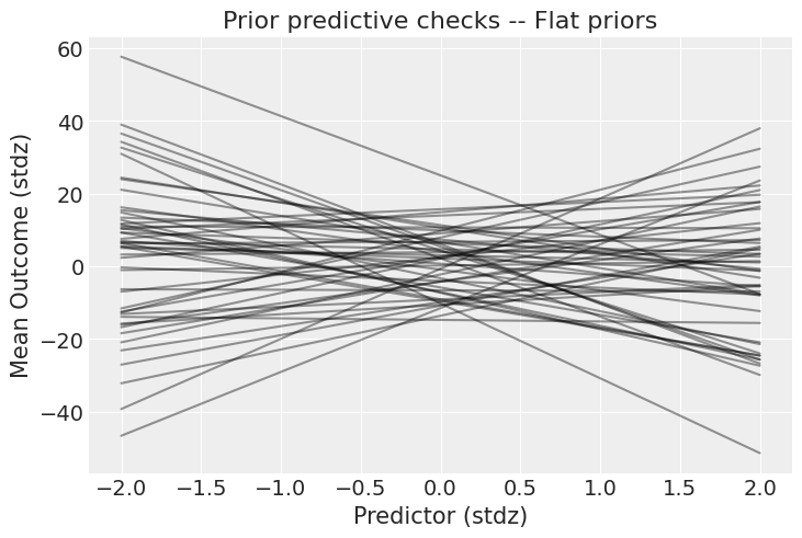
../../_images/ff23516dbee6a363a9666322f96566d04330e625e30db70966f6d9dd677d6f8d.png

这些先验允许结果和预测变量之间存在极其强的关系。当然，先验的选择始终取决于您的模型和数据，但请看 y 轴的刻度：结果可以从 -40 到 +40 个标准差（记住，数据是标准化的）。我希望您会同意这太宽松了——我们可以做得更好！让我们使用弱信息先验，看看它们会产生什么结果。在真实的案例研究中，这是您将科学知识融入到模型中的部分

with pm.Model() as model_1:
    a = pm.Normal("a", 0.0, 0.5)
    b = pm.Normal("b", 0.0, 1.0)

    mu = a + b * predictor_scaled
    sigma = pm.Exponential("sigma", 1.0)

    pm.Normal("obs", mu=mu, sigma=sigma, observed=outcome_scaled)
    idata = pm.sample_prior_predictive(draws=50, random_seed=rng)

Sampling: [a, b, obs, sigma]

_, ax = plt.subplots()

x = xr.DataArray(np.linspace(-2, 2, 50), dims=["plot_dim"])
prior = idata.prior
y = prior["a"] + prior["b"] * x

ax.plot(x, y.stack(sample=("chain", "draw")), c="k", alpha=0.4)

ax.set_xlabel("Predictor (stdz)")
ax.set_ylabel("Mean Outcome (stdz)")
ax.set_title("Prior predictive checks -- Weakly regularizing priors");

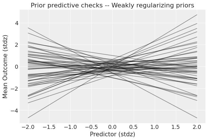
../../_images/f6a6c1116b9f7cb6da212ccfc15a084c5a93885194033931d659fa0c272a23d3.png

嗯，这好多了！仍然存在非常强的关系，但至少现在结果保持在可能的范围内。现在，是时候狂欢了——如果“狂欢”指的是“运行模型”，当然。

with model_1:
    idata.extend(pm.sample(1000, tune=2000, random_seed=rng))

az.plot_trace(idata);

Auto-assigning NUTS sampler...
Initializing NUTS using jitter+adapt_diag...
Multiprocess sampling (4 chains in 4 jobs)
NUTS: [a, b, sigma]

Sampling 4 chains for 2_000 tune and 1_000 draw iterations (8_000 + 4_000 draws total) took 14 seconds.

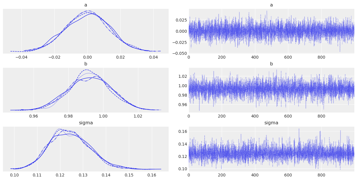
../../_images/c30ae812111d855935f054a90acba02cf89c774df6cfb0e6a5f08bccafb47b3e.png

一切运行顺利，但在分析轨迹图或表格摘要时，通常很难理解参数值的含义——在这里更是如此，因为参数存在于标准化空间中。理解您的模型的一个有用的方法是……您猜对了：后验预测检查！我们将使用 PyMC 的专用函数从后验分布中抽样数据。此函数将从轨迹中随机抽取 4000 个参数样本。然后，对于每个样本，它将从由该样本中 mu 和 sigma 的值指定的正态分布中抽取 100 个随机数

with model_1:
    pm.sample_posterior_predictive(idata, extend_inferencedata=True, random_seed=rng)

Sampling: [obs]

现在，idata 中的 posterior_predictive 组包含 4000 个生成的数据集（每个数据集包含 100 个样本），每个数据集都使用来自后验分布的不同参数设置

一种常见的可视化方法是查看模型是否可以重现真实数据中观察到的模式。 ArviZ 有一个非常简洁的函数可以开箱即用地做到这一点

az.plot_ppc(idata, num_pp_samples=100);

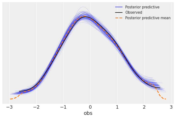
../../_images/fe93e1963079f236f472726d7e5a22241866b629391de65d433f6f3512ca6f01.png

看起来该模型在回溯预测数据方面做得相当好。除了这个通用函数之外，根据您的用例定制一个图表总是很不错的。在这里，绘制预测变量和结果之间预测的关系会很有趣。这非常容易，因为我们已经抽样了后验预测样本——我们只需要将参数传递到模型中即可

post = idata.posterior
mu_pp = post["a"] + post["b"] * xr.DataArray(predictor_scaled, dims=["obs_id"])

_, ax = plt.subplots()

ax.plot(
    predictor_scaled, mu_pp.mean(("chain", "draw")), label="Mean outcome", color="C1", alpha=0.6
)
ax.scatter(predictor_scaled, idata.observed_data["obs"])
az.plot_hdi(predictor_scaled, idata.posterior_predictive["obs"])

ax.set_xlabel("Predictor (stdz)")
ax.set_ylabel("Outcome (stdz)");

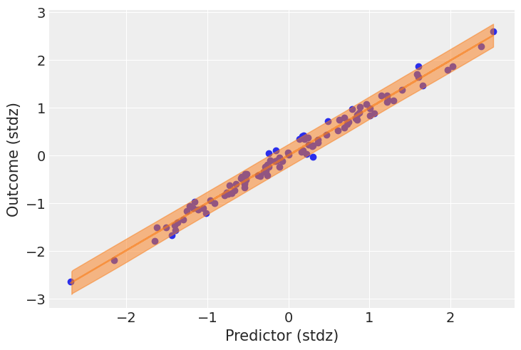
../../_images/3afe24e7b160465c730b0f96b00c980cb5d4e90b1529f656e2fdca57913d72ac.png

我们有很多数据，因此结果均值周围的不确定性非常小；但围绕结果的总体不确定性似乎与观察到的数据非常一致。

PPC 与其他模型评估方法之间的比较。#

关于这方面的出色介绍在 Edward 文档中给出

PPCs 是修订模型、简化或扩展当前模型的绝佳工具，因为它可以检查模型与数据的拟合程度。它们的灵感来自先验检查和经典假设检验，其理念是应该在大量样本评估的频率论视角下批评模型。

PPCs 也可以应用于假设检验、模型比较、模型选择和模型平均等任务。重要的是要注意，虽然它们可以作为贝叶斯假设检验的一种形式应用，但通常不建议进行假设检验：从单个测试中进行二元决策并不像人们可能认为的那样常见。我们建议执行许多 PPC，以全面了解模型的拟合度。

预测#

相同的模式可以用于预测。在这里，我们正在构建一个逻辑回归模型

N = 400
true_intercept = 0.2
true_slope = 1.0
predictors = rng.normal(size=N)
true_p = logistic(true_intercept + true_slope * predictors)

outcomes = rng.binomial(1, true_p)
outcomes[:10]

array([1, 1, 1, 0, 1, 0, 0, 1, 1, 0])

with pm.Model() as model_2:
    betas = pm.Normal("betas", mu=0.0, sigma=np.array([0.5, 1.0]), shape=2)

    # set predictors as shared variable to change them for PPCs:
    pred = pm.MutableData("pred", predictors, dims="obs_id")
    p = pm.Deterministic("p", pm.math.invlogit(betas[0] + betas[1] * pred), dims="obs_id")

    outcome = pm.Bernoulli("outcome", p=p, observed=outcomes, dims="obs_id")

    idata_2 = pm.sample(1000, tune=2000, return_inferencedata=True, random_seed=rng)
az.summary(idata_2, var_names=["betas"], round_to=2)

/home/ricardo/Documents/Projects/pymc/pymc/data.py:304: FutureWarning: MutableData is deprecated. All Data variables are now mutable. Use Data instead.
  warnings.warn(
Auto-assigning NUTS sampler...
Initializing NUTS using jitter+adapt_diag...
Multiprocess sampling (4 chains in 4 jobs)
NUTS: [betas]

Sampling 4 chains for 2_000 tune and 1_000 draw iterations (8_000 + 4_000 draws total) took 6 seconds.

	mean	sd	hdi_3%	hdi_97%	mcse_mean	mcse_sd	ess_bulk	ess_tail	r_hat
betas[0]	0.23	0.11	0.03	0.44	0.0	0.0	3211.49	3013.30	1.0
betas[1]	1.03	0.13	0.78	1.29	0.0	0.0	3673.85	2720.49	1.0

现在，让我们模拟样本外数据，看看模型如何预测它们。我们将新的预测变量提供给模型，然后它会根据在训练轮中学到的内容告诉我们它认为结果是什么。然后，我们将模型的预测与真实的样本外结果进行比较。

predictors_out_of_sample = rng.normal(size=50)
outcomes_out_of_sample = rng.binomial(
    1, logistic(true_intercept + true_slope * predictors_out_of_sample)
)

with model_2:
    # update values of predictors:
    pm.set_data({"pred": predictors_out_of_sample})
    # use the updated values and predict outcomes and probabilities:
    idata_2 = pm.sample_posterior_predictive(
        idata_2,
        var_names=["p"],
        return_inferencedata=True,
        predictions=True,
        extend_inferencedata=True,
        random_seed=rng,
    )

Sampling: []

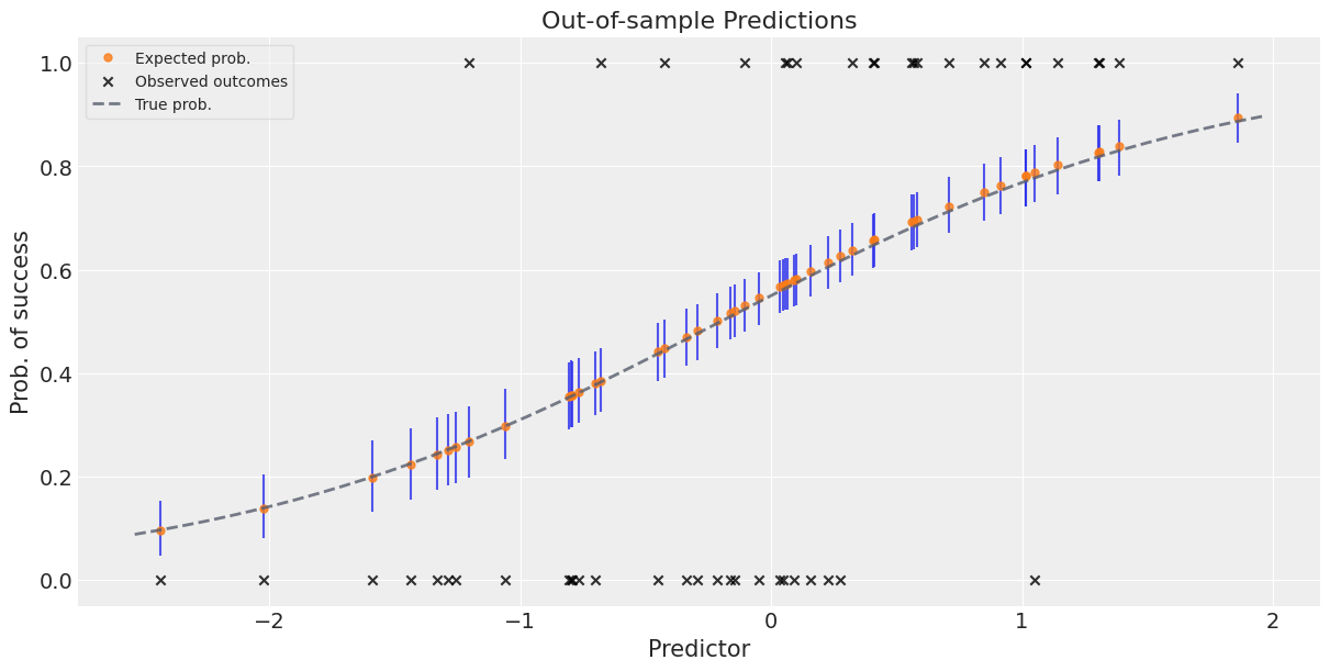
平均预测值加上误差条，以给出预测不确定性的感觉#

请注意，由于我们正在处理完整的后验分布，因此我们也可以免费获得预测中的不确定性。

_, ax = plt.subplots(figsize=(12, 6))

preds_out_of_sample = idata_2.predictions_constant_data.sortby("pred")["pred"]
model_preds = idata_2.predictions.sortby(preds_out_of_sample)

# uncertainty about the estimates:
ax.vlines(
    preds_out_of_sample,
    *az.hdi(model_preds)["p"].transpose("hdi", ...),
    alpha=0.8,
)
# expected probability of success:
ax.plot(
    preds_out_of_sample,
    model_preds["p"].mean(("chain", "draw")),
    "o",
    ms=5,
    color="C1",
    alpha=0.8,
    label="Expected prob.",
)

# actual outcomes:
ax.scatter(
    x=predictors_out_of_sample,
    y=outcomes_out_of_sample,
    marker="x",
    color="k",
    alpha=0.8,
    label="Observed outcomes",
)
# true probabilities:
x = np.linspace(predictors_out_of_sample.min() - 0.1, predictors_out_of_sample.max() + 0.1)
ax.plot(
    x,
    logistic(true_intercept + true_slope * x),
    lw=2,
    ls="--",
    color="#565C6C",
    alpha=0.8,
    label="True prob.",
)

ax.set_xlabel("Predictor")
ax.set_ylabel("Prob. of success")
ax.set_title("Out-of-sample Predictions")
ax.legend(fontsize=10, frameon=True, framealpha=0.5);

../../_images/b84d7054a68a06b9a9d462a4c1b44bb826b4c04b3c0b855b99fc794af87610f6.png

%load_ext watermark
%watermark -n -u -v -iv -w -p pytensor

Last updated: Tue Jun 25 2024

Python implementation: CPython
Python version       : 3.11.8
IPython version      : 8.22.2

pytensor: 2.20.0+3.g66439d283.dirty

pymc      : 5.15.0+1.g58927d608
numpy     : 1.26.4
arviz     : 0.17.1
matplotlib: 3.8.3
xarray    : 2024.2.0

Watermark: 2.4.3