PyMC 和 PyTensor#
作者: Ricardo Vieira 和 Juan Orduz
在本笔记本中,我们希望介绍 PyMC 模型如何转换为 PyTensor 图。目的不是详细描述所有 pytensor 的功能,而是侧重于理解其与 PyMC 连接的主要概念。有关该项目的更详细描述,请参阅官方文档。
准备笔记本#
首先导入所需的库。
import matplotlib.pyplot as plt
import numpy as np
import pytensor
import pytensor.tensor as pt
import scipy.stats

import pymc as pm
PyTensor 简介#
我们首先研究 pytensor。根据他们的文档
PyTensor 是一个 Python 库,允许用户定义、优化和高效评估涉及多维数组的数学表达式。

一个简单的例子#
首先,我们定义一些 pytensor 张量,并展示如何执行一些基本操作。
x = pt.scalar(name="x")
y = pt.vector(name="y")

print(
    f"""
x type: {x.type}
x name = {x.name}
---
y type: {y.type}
y name = {y.name}
"""
)
x type: Scalar(float64, shape=())
x name = x
---
y type: Vector(float64, shape=(?,))
y name = y
现在我们已经定义了 x 和 y 张量,我们可以通过将它们加在一起来创建一个新的张量。
z = x + y
z.name = "x + y"
为了使计算稍微复杂一些,让我们取结果张量的对数。
w = pt.log(z)
w.name = "log(x + y)"
我们可以使用 dprint() 函数来打印任何给定张量的计算图。
pytensor.dprint(w)
Log [id A] 'log(x + y)'
 └─ Add [id B] 'x + y'
    ├─ ExpandDims{axis=0} [id C]
    │  └─ x [id D]
    └─ y [id E]
<ipykernel.iostream.OutStream at 0x7fc6cd274a90>
请注意,此图不执行任何计算(尚未!)。它只是定义要执行的步骤序列。我们可以使用 function() 来定义一个可调用对象,以便我们可以将值推送到图中。
f = pytensor.function(inputs=[x, y], outputs=w)
现在图已编译,我们可以推送一些具体的值
f(x=0, y=[1, np.e])
array([0., 1.])
提示
有时我们只想调试,我们可以使用 eval() 来实现
w.eval({x: 0, y: [1, np.e]})
array([0., 1.])
您也可以设置中间值
w.eval({z: [1, np.e]})
array([0., 1.])
PyTensor 很聪明!#
pytensor 最重要的功能之一是它可以自动优化图内的数学运算。让我们考虑一个简单的例子
a = pt.scalar(name="a")
b = pt.scalar(name="b")

c = a / b
c.name = "a / b"

pytensor.dprint(c)
True_div [id A] 'a / b'
 ├─ a [id B]
 └─ b [id C]
<ipykernel.iostream.OutStream at 0x7fc6cd274a90>
现在让我们将 b 乘以 c。这应该简单地得到 a。
d = b * c
d.name = "b * c"

pytensor.dprint(d)
Mul [id A] 'b * c'
 ├─ b [id B]
 └─ True_div [id C] 'a / b'
    ├─ a [id D]
    └─ b [id B]
<ipykernel.iostream.OutStream at 0x7fc6cd274a90>
该图显示了完整的计算,但是一旦我们编译它,该操作就变成了 a 上的恒等式,正如预期的那样。
g = pytensor.function(inputs=[a, b], outputs=d)

pytensor.dprint(g)
DeepCopyOp [id A] 0
 └─ a [id B]
<ipykernel.iostream.OutStream at 0x7fc6cd274a90>
PyTensor 图中有什么?#
下图显示了 pytensor 图的基本结构。
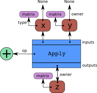
我们可以通过在上面章节的第一个示例中显式指示这些概念,使这些概念更具体。让我们计算张量 z 的图组件。
print(
    f"""
z type: {z.type}
z name = {z.name}
z owner = {z.owner}
z owner inputs = {z.owner.inputs}
z owner op = {z.owner.op}
z owner output = {z.owner.outputs}
"""
)
z type: Vector(float64, shape=(?,))
z name = x + y
z owner = Add(ExpandDims{axis=0}.0, y)
z owner inputs = [ExpandDims{axis=0}.0, y]
z owner op = Add
z owner output = [x + y]
以下代码片段通过遍历 w 的计算图,帮助我们理解这些概念。实际代码在这里并不重要,重点是输出。
# start from the top
stack = [w]

while stack:
    print("---")
    var = stack.pop(0)
    print(f"Checking variable {var} of type {var.type}")
    # check variable is not a root variable
    if var.owner is not None:
        print(f" > Op is {var.owner.op}")
        # loop over the inputs
        for i, input in enumerate(var.owner.inputs):
            print(f" > Input {i} is {input}")
            stack.append(input)
    else:
        print(f" > {var} is a root variable")
---
Checking variable log(x + y) of type Vector(float64, shape=(?,))
 > Op is Log
 > Input 0 is x + y
---
Checking variable x + y of type Vector(float64, shape=(?,))
 > Op is Add
 > Input 0 is ExpandDims{axis=0}.0
 > Input 1 is y
---
Checking variable ExpandDims{axis=0}.0 of type Vector(float64, shape=(1,))
 > Op is ExpandDims{axis=0}
 > Input 0 is x
---
Checking variable y of type Vector(float64, shape=(?,))
 > y is a root variable
---
Checking variable x of type Scalar(float64, shape=())
 > x is a root variable
请注意,这与上面介绍的 dprint() 函数的输出非常相似。
pytensor.dprint(w)
Log [id A] 'log(x + y)'
 └─ Add [id B] 'x + y'
    ├─ ExpandDims{axis=0} [id C]
    │  └─ x [id D]
    └─ y [id E]
<ipykernel.iostream.OutStream at 0x7fc6cd274a90>
图操作 101#
PyTensor 的另一个有趣功能是能够操作计算图,这在 TensorFlow 或 PyTorch 中是不可能的。在这里,我们继续上面的示例,以说明围绕此技术的主要思想。
# get input tensors
list(pytensor.graph.graph_inputs(graphs=[w]))
[x, y]
作为一个简单的示例,让我们在 exp() 之前添加一个 log()(以获得恒等函数)。
parent_of_w = w.owner.inputs[0]  # get z tensor
new_parent_of_w = pt.exp(parent_of_w)  # modify the parent of w
new_parent_of_w.name = "exp(x + y)"
请注意,w 的图实际上没有改变
pytensor.dprint(w)
Log [id A] 'log(x + y)'
 └─ Add [id B] 'x + y'
    ├─ ExpandDims{axis=0} [id C]
    │  └─ x [id D]
    └─ y [id E]
<ipykernel.iostream.OutStream at 0x7fc6cd274a90>
要修改图,我们需要使用 clone_replace() 函数,该函数返回初始子图的副本,并进行相应的替换。
new_w = pytensor.clone_replace(output=[w], replace={parent_of_w: new_parent_of_w})[0]
new_w.name = "log(exp(x + y))"
pytensor.dprint(new_w)
Log [id A] 'log(exp(x + y))'
 └─ Exp [id B] 'exp(x + y)'
    └─ Add [id C] 'x + y'
       ├─ ExpandDims{axis=0} [id D]
       │  └─ x [id E]
       └─ y [id F]
<ipykernel.iostream.OutStream at 0x7fc6cd274a90>
最后,我们可以通过将一些输入传递到新图中来测试修改后的图。
new_w.eval({x: 0, y: [1, np.e]})
array([1. , 2.71828183])
正如预期的那样,新图只是恒等函数。
注意
再次注意,pytensor 非常聪明,足以在编译函数后省略 exp 和 log。
f = pytensor.function(inputs=[x, y], outputs=new_w)

pytensor.dprint(f)
Add [id A] 'x + y' 1
 ├─ ExpandDims{axis=0} [id B] 0
 │  └─ x [id C]
 └─ y [id D]
<ipykernel.iostream.OutStream at 0x7fc6cd274a90>
f(x=0, y=[1, np.e])
array([1. , 2.71828183])
PyTensor RandomVariables#
现在我们已经了解了 pytensor 的基础知识,我们希望朝着随机变量的方向发展。
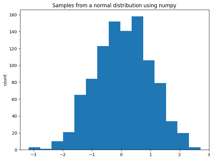
我们如何在 numpy 中生成随机数?为了说明这一点,我们可以从正态分布中采样
a = np.random.normal(loc=0, scale=1, size=1_000)

fig, ax = plt.subplots(figsize=(8, 6))
ax.hist(a, color="C0", bins=15)
ax.set(title="Samples from a normal distribution using numpy", ylabel="count");
现在让我们尝试在 PyTensor 中执行此操作。
y = pt.random.normal(loc=0, scale=1, name="y")
y.type
TensorType(float64, shape=())
接下来,我们使用 dprint() 显示该图。
pytensor.dprint(y)
normal_rv{"(),()->()"}.1 [id A] 'y'
 ├─ RNG(<Generator(PCG64) at 0x7FC6504CC740>) [id B]
 ├─ NoneConst{None} [id C]
 ├─ 0 [id D]
 └─ 1 [id E]
<ipykernel.iostream.OutStream at 0x7fc6cd274a90>
输入始终按以下顺序排列
rng共享变量大小arg1arg2argn
我们可以通过在随机变量上调用 eval() 来进行采样。
y.eval()
array(0.67492335)
但是请注意,这些样本始终相同!
for i in range(10):
    print(f"Sample {i}: {y.eval()}")
Sample 0: 0.6749233482557402
Sample 1: 0.6749233482557402
Sample 2: 0.6749233482557402
Sample 3: 0.6749233482557402
Sample 4: 0.6749233482557402
Sample 5: 0.6749233482557402
Sample 6: 0.6749233482557402
Sample 7: 0.6749233482557402
Sample 8: 0.6749233482557402
Sample 9: 0.6749233482557402
我们总是得到相同的样本!这与图中的随机种子步骤有关,即 RandomGeneratorSharedVariable(我们在此处不深入探讨此主题)。我们将在下面展示如何使用 pymc 生成不同的样本。
PyMC#

为此,我们首先定义一个 pymc 正态分布。
x = pm.Normal.dist(mu=0, sigma=1)
pytensor.dprint(x)
normal_rv{"(),()->()"}.1 [id A]
 ├─ RNG(<Generator(PCG64) at 0x7FC650553D80>) [id B]
 ├─ NoneConst{None} [id C]
 ├─ 0 [id D]
 └─ 1 [id E]
<ipykernel.iostream.OutStream at 0x7fc6cd274a90>
观察到 x 只是一个正态 RandomVariable,它与 y 相同,除了 rng。
我们可以尝试像上面一样通过调用 eval() 来生成样本。
for i in range(10):
    print(f"Sample {i}: {x.eval()}")
Sample 0: 0.3880069666747013
Sample 1: 0.3880069666747013
Sample 2: 0.3880069666747013
Sample 3: 0.3880069666747013
Sample 4: 0.3880069666747013
Sample 5: 0.3880069666747013
Sample 6: 0.3880069666747013
Sample 7: 0.3880069666747013
Sample 8: 0.3880069666747013
Sample 9: 0.3880069666747013
和以前一样,我们在所有迭代中都得到相同的值。生成随机样本的正确方法是使用 draw()。
fig, ax = plt.subplots(figsize=(8, 6))
ax.hist(pm.draw(x, draws=1_000), color="C1", bins=15)
ax.set(title="Samples from a normal distribution using pymc", ylabel="count");
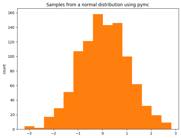
耶!我们学会了如何从 pymc 分布中采样!
幕后发生了什么?#
我们现在可以研究如何在 Model 内部完成此操作。
with pm.Model() as model:
    z = pm.Normal(name="z", mu=np.array([0, 0]), sigma=np.array([1, 2]))

pytensor.dprint(z)
normal_rv{"(),()->()"}.1 [id A] 'z'
 ├─ RNG(<Generator(PCG64) at 0x7FC6482D1FC0>) [id B]
 ├─ NoneConst{None} [id C]
 ├─ [0 0] [id D]
 └─ [1 2] [id E]
<ipykernel.iostream.OutStream at 0x7fc6cd274a90>
我们只是像之前看到的那样创建随机变量,但现在将它们注册到 pymc 模型中。要提取随机变量列表,我们可以简单地执行
model.basic_RVs
[z ~ Normal(<constant>, <constant>)]
pytensor.dprint(model.basic_RVs[0])
normal_rv{"(),()->()"}.1 [id A] 'z'
 ├─ RNG(<Generator(PCG64) at 0x7FC6482D1FC0>) [id B]
 ├─ NoneConst{None} [id C]
 ├─ [0 0] [id D]
 └─ [1 2] [id E]
<ipykernel.iostream.OutStream at 0x7fc6cd274a90>
我们可以尝试像上面一样通过 eval() 进行采样,并且毫不奇怪,我们在每次迭代中都获得相同的样本。
for i in range(10):
    print(f"Sample {i}: {z.eval()}")
Sample 0: [-0.78480847  2.20329511]
Sample 1: [-0.78480847  2.20329511]
Sample 2: [-0.78480847  2.20329511]
Sample 3: [-0.78480847  2.20329511]
Sample 4: [-0.78480847  2.20329511]
Sample 5: [-0.78480847  2.20329511]
Sample 6: [-0.78480847  2.20329511]
Sample 7: [-0.78480847  2.20329511]
Sample 8: [-0.78480847  2.20329511]
Sample 9: [-0.78480847  2.20329511]
同样,正确的采样方法是通过 draw()。
for i in range(10):
    print(f"Sample {i}: {pm.draw(z)}")
Sample 0: [-1.10363734 -4.33735303]
Sample 1: [ 0.69639479 -0.81137315]
Sample 2: [ 1.25238284 -0.0119145 ]
Sample 3: [ 1.21683809 -3.08878544]
Sample 4: [1.63496743 2.58329782]
Sample 5: [0.4128748  3.29810689]
Sample 6: [1.76074607 3.33727713]
Sample 7: [ 0.92855273 -0.14005723]
Sample 8: [ 2.04166261 -1.25987621]
Sample 9: [-0.24230627 -2.91013171]
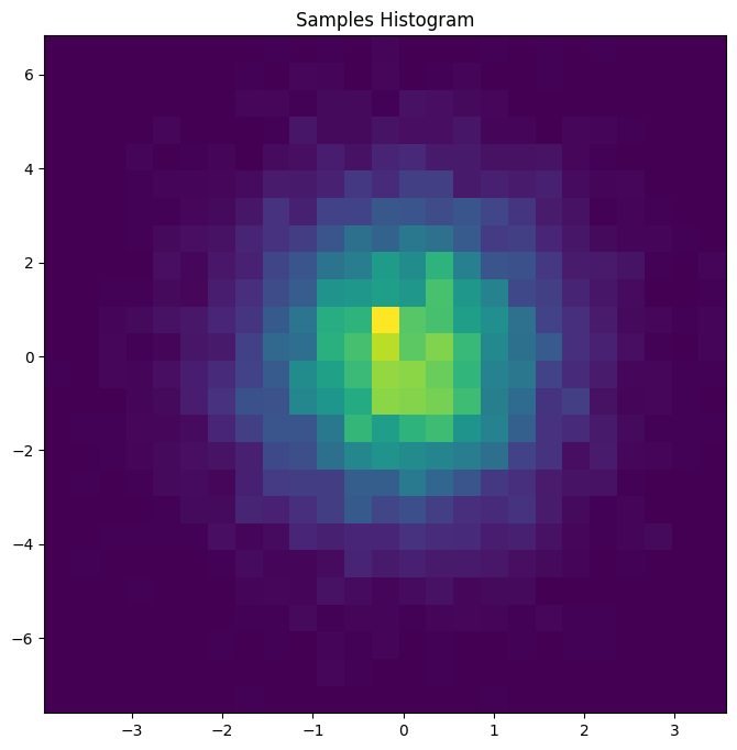
fig, ax = plt.subplots(figsize=(8, 8))
z_draws = pm.draw(vars=z, draws=10_000)
ax.hist2d(x=z_draws[:, 0], y=z_draws[:, 1], bins=25)
ax.set(title="Samples Histogram");
随机变量够了,我想看一些(对数)概率!#
回想一下,我们在上面定义了以下模型
model
pymc 能够将 RandomVariable 转换为它们各自的概率函数。一种简单的方法是使用 logp(),它将 RandomVariable 作为第一个输入,并将评估 logp 的值作为第二个输入(我们将在稍后更详细地讨论这一点)。
z_value = pt.vector(name="z")
z_logp = pm.logp(rv=z, value=z_value)
z_logp 包含 PyTensor 图,该图表示在 z_value 处评估的正态随机变量 z 的对数概率。
pytensor.dprint(z_logp)
Check{sigma > 0} [id A] 'z_logprob'
 ├─ Sub [id B]
 │  ├─ Sub [id C]
 │  │  ├─ Mul [id D]
 │  │  │  ├─ ExpandDims{axis=0} [id E]
 │  │  │  │  └─ -0.5 [id F]
 │  │  │  └─ Pow [id G]
 │  │  │     ├─ True_div [id H]
 │  │  │     │  ├─ Sub [id I]
 │  │  │     │  │  ├─ z [id J]
 │  │  │     │  │  └─ [0 0] [id K]
 │  │  │     │  └─ [1 2] [id L]
 │  │  │     └─ ExpandDims{axis=0} [id M]
 │  │  │        └─ 2 [id N]
 │  │  └─ ExpandDims{axis=0} [id O]
 │  │     └─ Log [id P]
 │  │        └─ Sqrt [id Q]
 │  │           └─ 6.283185307179586 [id R]
 │  └─ Log [id S]
 │     └─ [1 2] [id L]
 └─ All{axes=None} [id T]
    └─ MakeVector{dtype='bool'} [id U]
       └─ All{axes=None} [id V]
          └─ Gt [id W]
             ├─ [1 2] [id L]
             └─ ExpandDims{axis=0} [id X]
                └─ 0 [id Y]
<ipykernel.iostream.OutStream at 0x7fc6cd274a90>
提示
还有一个方便的 pymc 函数来计算随机变量 logcdf() 的对数累积概率。
请注意,正如开头所解释的,尚未进行任何计算。实际计算是在编译并传递输入后执行的。仅出于说明目的,我们将再次使用方便的 eval() 方法。
z_logp.eval({z_value: [0, 0]})
array([-0.91893853, -1.61208571])
这仅仅是评估正态分布的对数概率。
scipy.stats.norm.logpdf(x=np.array([0, 0]), loc=np.array([0, 0]), scale=np.array([1, 2]))
array([-0.91893853, -1.61208571])
pymc 模型提供了一些有用的例程,以方便将 RandomVariable 转换为概率函数。例如,logp() 可以用于提取模型中所有变量的联合概率
pytensor.dprint(model.logp(sum=False))
Check{sigma > 0} [id A] 'z_logprob'
 ├─ Sub [id B]
 │  ├─ Sub [id C]
 │  │  ├─ Mul [id D]
 │  │  │  ├─ ExpandDims{axis=0} [id E]
 │  │  │  │  └─ -0.5 [id F]
 │  │  │  └─ Pow [id G]
 │  │  │     ├─ True_div [id H]
 │  │  │     │  ├─ Sub [id I]
 │  │  │     │  │  ├─ z [id J]
 │  │  │     │  │  └─ [0 0] [id K]
 │  │  │     │  └─ [1 2] [id L]
 │  │  │     └─ ExpandDims{axis=0} [id M]
 │  │  │        └─ 2 [id N]
 │  │  └─ ExpandDims{axis=0} [id O]
 │  │     └─ Log [id P]
 │  │        └─ Sqrt [id Q]
 │  │           └─ 6.283185307179586 [id R]
 │  └─ Log [id S]
 │     └─ [1 2] [id L]
 └─ All{axes=None} [id T]
    └─ MakeVector{dtype='bool'} [id U]
       └─ All{axes=None} [id V]
          └─ Gt [id W]
             ├─ [1 2] [id L]
             └─ ExpandDims{axis=0} [id X]
                └─ 0 [id Y]
<ipykernel.iostream.OutStream at 0x7fc6cd274a90>
由于我们只有一个变量,因此此函数等效于我们之前手动调用 pm.logp 获得的结果。我们还可以使用辅助函数 compile_logp() 来返回模型 logp 的已编译 PyTensor 函数。
logp_function = model.compile_logp(sum=False)
此函数需要一个“点”字典作为输入。我们可以自己创建它,但为了说明另一个有用的 Model 方法,让我们调用 initial_point(),它返回大多数采样器在决定从哪里开始采样时使用的点。
point = model.initial_point()
point
{'z': array([0., 0.])}
logp_function(point)
[array([-0.91893853, -1.61208571])]
什么是值变量,为什么它们很重要?#
正如我们在上面看到的,logp 图没有随机变量。相反,它是根据输入(值)变量定义的。当我们想要采样时,每个随机变量 (RV) 都被在各自的输入(值)变量处评估的 logp 函数替换。让我们通过一些示例看看这是如何工作的。RV 和值变量可以在这些 scipy 操作中观察到
rv = scipy.stats.norm(0, 1)

# Equivalent to rv = pm.Normal("rv", 0, 1)
scipy.stats.norm(0, 1)
<scipy.stats._distn_infrastructure.rv_continuous_frozen at 0x7fc64808be10>
# Equivalent to rv_draw = pm.draw(rv, 3)
rv.rvs(3)
array([-1.00721939, -0.60656542, -0.28202337])
# Equivalent to rv_logp = pm.logp(rv, 1.25)
rv.logpdf(1.25)
-1.7001885332046727
接下来,让我们看看这些值变量在稍微复杂的模型中的行为。
with pm.Model() as model_2:
    mu = pm.Normal(name="mu", mu=0, sigma=2)
    sigma = pm.HalfNormal(name="sigma", sigma=3)
    x = pm.Normal(name="x", mu=mu, sigma=sigma)
每个模型 RV 都与一个“值变量”相关
model_2.rvs_to_values
{mu ~ Normal(0, 2): mu,
 sigma ~ HalfNormal(0, 3): sigma_log__,
 x ~ Normal(mu, sigma): x}
请注意,对于 sigma,关联值在对数刻度中,因为实际上我们需要 NUTS 采样的无界值。
model_2.value_vars
[mu, sigma_log__, x]
现在我们知道了如何提取模型变量,我们可以计算特定值的模型元素级对数概率。
# extract values as pytensor.tensor.var.TensorVariable
mu_value = model_2.rvs_to_values[mu]
sigma_log_value = model_2.rvs_to_values[sigma]
x_value = model_2.rvs_to_values[x]
# element-wise log-probability of the model (we do not take te sum)
logp_graph = pt.stack(model_2.logp(sum=False))
# evaluate by passing concrete values
logp_graph.eval({mu_value: 0, sigma_log_value: -10, x_value: 0})
array([ -1.61208572, -11.32440366, 9.08106147])
这等效于
print(
    f"""
mu_value -> {scipy.stats.norm.logpdf(x=0, loc=0, scale=2)}
sigma_log_value -> {-10 + scipy.stats.halfnorm.logpdf(x=np.exp(-10), loc=0, scale=3)}
x_value -> {scipy.stats.norm.logpdf(x=0, loc=0, scale=np.exp(-10))}
"""
)
mu_value -> -1.612085713764618
sigma_log_value -> -11.324403641427345
x_value -> 9.081061466795328
注意
对于 sigma_log_value,我们添加 \(-10\) 项,使 scipy 和 pytensor 匹配,这是因为雅可比矩阵。
正如我们已经看到的,我们还可以使用方法 compile_logp() 来获得模型 logp 的已编译 pytensor 函数,该函数将 {值变量名称 : 值} 字典作为输入
model_2.compile_logp(sum=False)({"mu": 0, "sigma_log__": -10, "x": 0})
[array(-1.61208572), array(-11.32440366), array(9.08106147)]
Model 类还具有提取 logp 的梯度 (dlogp()) 和 hessian (d2logp()) 的方法。
如果您想更深入地了解 pytensor RandomVariables 和 pymc 分布的内部原理,请查看 分布开发者指南。
%load_ext watermark
%watermark -n -u -v -iv -w -p pytensor
Last updated: Tue Jun 25 2024

Python implementation: CPython
Python version       : 3.11.8
IPython version      : 8.22.2

pytensor: 2.20.0+3.g66439d283.dirty

pytensor  : 2.20.0+3.g66439d283.dirty
pymc      : 5.15.0+1.g58927d608
scipy     : 1.12.0
numpy     : 1.26.4
matplotlib: 3.8.3

Watermark: 2.4.3