


用于制作个性化推荐的概率矩阵分解#
import arviz as az
import matplotlib.pyplot as plt
import numpy as np
import pandas as pd
import pymc as pm
import xarray as xr
%config InlineBackend.figure_format = 'retina'
RANDOM_SEED = 8927
rng = np.random.default_rng(RANDOM_SEED)
az.style.use("arviz-darkgrid")
动机#
假设您正在 Netflix 上浏览想看的内容,但就是不喜欢这些建议。您只是知道您可以做得更好。您只需要从自己和朋友那里收集一些评分数据,然后构建一个推荐算法。本笔记本将指导您完成这项工作!
我们将从对我们的模型如何工作有一些直观的了解开始。然后我们将形式化我们的直觉。之后,我们将检查我们要使用的数据集。一旦我们对数据的外观有了一些概念,我们将定义一些预测电影偏好的基线方法。接下来,我们将研究概率矩阵分解 (PMF),这是一种更复杂的贝叶斯方法,用于预测偏好。详细介绍了 PMF 模型后,我们将使用 PyMC 进行 MAP 估计和 MCMC 推断。最后,我们将比较使用 PMF 获得的结果与从我们的基线方法获得的结果,并讨论结果。
直觉#
通常,如果我们想要获得某些东西的推荐,我们会尝试找到与我们相似的人并征求他们的意见。如果 Bob、Alice 和 Monty 都和我相似,并且他们都喜欢犯罪剧,那么我也可能会喜欢犯罪剧。但这并非总是如此。这取决于我们认为什么是“相似”。为了获得最佳效果,我们真正想寻找的是品味最相似的人。品味是一种复杂的野兽,我们可能想将其分解为更容易理解的东西。我们可能会尝试根据各种因素来描述每部电影。也许电影可以是情绪化的、轻松愉快的、电影化的、对话密集的、大预算的等等。现在想象一下,我们浏览 IMDB 并为每部电影在每个类别中分配一个评分。它的情绪化程度如何?它有多少对话?它的预算是多少?也许我们对每个类别使用 0 到 1 之间的数字。直观地,我们可能会称之为电影的概况。
现在假设我们回到我们评分的那 5 部电影。此时,我们可以通过查看我们喜欢和不喜欢的每部电影的电影概况,更丰富地了解我们自己的偏好。也许我们取这 5 部电影概况的平均值,并称之为我们理想的电影类型。换句话说,我们已经计算出了一些我们对各种类型电影的内在偏好的概念。假设 Bob、Alice 和 Monty 都做了同样的事情。现在我们可以比较我们的偏好,并确定我们每个人真正有多相似。我可能会发现 Bob 是最相似的,而另外两个人仍然比其他人更相似,但不如 Bob 那么相似。因此,我想要来自所有三个人的推荐,但是当我做出最终决定时,我会更重视 Bob 的推荐,而不是我从 Alice 和 Monty 那里得到的推荐。
虽然上述过程听起来相当有效,但它也揭示了一个意想不到的额外信息来源。如果我们对某部特定的电影给予了高度评价,并且我们知道它的电影概况,我们可以与其他电影的概况进行比较。如果我们找到一部数字非常接近的电影,我们也很可能喜欢这部电影。这两种方法以及上面的方法通常被称为邻域方法。同时利用这两种方法的技术通常称为协同过滤 [Koren et al., 2009]。我们谈到的第一种方法使用用户-用户相似度,而第二种方法使用项目-项目相似度。理想情况下,我们希望同时使用这两种信息来源。我们的想法是我们有很多项目可供选择,并且我们希望与其他人合作,将项目列表过滤到我们每个人最喜欢的项目。我的列表应该将我最喜欢的项目放在顶部,而将我最不喜欢的项目放在底部。其他每个人都想要同样的东西。如果我与一群其他人聚在一起,我们都看了 5 部电影,并且我们有一些有效的计算过程来确定相似度,我们可以非常快速地按我们的喜好对电影进行排序。
形式化#
让我们花一些时间使我们一直在讨论的直观概念更加具体。我们有一组 \(M\) 部电影,或项目(在上面的示例中 \(M = 100\))。我们还有 \(N\) 个人,我们将其称为我们的推荐系统的用户。对于每个项目,我们都想找到一个 \(D\) 维因子组成(上面的电影概况)来描述该项目。理想情况下,我们希望在不实际手动标记所有电影的情况下做到这一点。手动标记既缓慢又容易出错,因为不同的人可能会以不同的方式标记电影。因此,我们将每部电影建模为一个 \(D\) 维向量,即其潜在因子组成。此外,我们期望每个用户都有一些偏好,但是如果没有我们的手动标记和平均过程,我们必须依靠潜在因子组成来学习每个用户的 \(D\) 维潜在偏好向量。我们唯一可以观察到的是用户提供的 \(N \times M\) 评分矩阵 \(R\)。条目 \(R_{ij}\) 是用户 \(i\) 对项目 \(j\) 的评分。这些条目中的许多条目可能缺失,因为大多数用户不会对所有 100 部电影进行评分。我们的目标是用基于潜在变量 \(U\) 和 \(V\) 的预测评分来填充缺失值。我们将预测评分表示为 \(R_{ij}^*\)。我们还定义了一个指示矩阵 \(I\),如果 \(R_{ij}\) 缺失,则条目 \(I_{ij} = 0\),否则 \(I_{ij} = 1\)。
因此,我们有一个 \(N \times D\) 用户偏好矩阵,我们将其称为 \(U\),以及一个 \(M \times D\) 因子组成矩阵,我们将其称为 \(V\)。我们还有一个 \(N \times M\) 评分矩阵,我们将其称为 \(R\)。我们可以将每一行 \(U_i\) 视为指示每个用户对 \(D\) 个潜在因子的偏好程度。每一行 \(V_j\) 可以被认为是每个项目在多大程度上可以用每个潜在因子来描述。为了提出建议,我们需要一个合适的预测函数,该函数将用户偏好向量 \(U_i\) 和项目潜在因子向量 \(V_j\) 映射到预测排名。此预测函数的选择是一个重要的建模决策,并且已经使用了各种预测函数。也许最常见的是两个向量的点积,\(U_i \cdot V_j\) [Koren et al., 2009]。
为了更好地理解 CF 技术,让我们探讨一个具体的例子。假设我们正在寻求使用一个模型来推荐电影,该模型推断五个潜在因子,\(V_j\),其中 \(j = 1,2,3,4,5\)。实际上,潜在因子通常无法以直接的方式解释,并且大多数模型都不会尝试理解每个因子捕获的信息。但是,为了解释的目的,让我们假设这五个潜在因子最终可能会捕获我们上面讨论的电影概况。因此,我们的五个潜在因子是:情绪化、轻松愉快、电影化、对话和预算。然后,对于特定的用户 \(i\),假设我们推断出一个偏好向量 \(U_i = <0.5, 0.1, 1.5, 1.1, 0.3>\)。此外,对于特定的项目 \(j\),我们推断出这些潜在因子的值:\(V_j = <0.5, 1.5, 1.25, 0.8, 0.9>\)。使用点积作为预测函数,我们将计算出 3.425 作为该项目的排名,考虑到我们的 1 到 5 评分等级,这或多或少是一种中性偏好。
数据#
MovieLens 100k 数据集 [Harper and Konstan, 2016] 由明尼苏达大学的 GroupLens 研究项目收集。该数据集包含来自 943 位用户对 1682 部电影的 100,000 个评分(1-5)。每位用户至少对 20 部电影进行了评分,并且具有关于用户的基本信息(年龄、性别、职业、邮政编码)。每部电影都包含基本信息,如标题、发行日期、视频发行日期和类型。我们将实施一个适用于此数据的协同过滤模型,并根据均方根误差 (RMSE) 对其进行评估,以验证结果。
数据是通过 MovieLens 网站 在 1997 年 9 月 19 日至 1998 年 4 月 22 日的七个月期间收集的。此数据已清理 - 评分少于 20 个或没有完整人口统计信息的用户已从此数据集中删除。
让我们从探索我们的数据开始。我们想对它的外观有一个大致的了解,并了解它可能包含哪些类型的模式。以下是用户评分数据
data_kwargs = dict(sep="\t", names=["userid", "itemid", "rating", "timestamp"])
try:
    data = pd.read_csv("../data/ml_100k_u.data", **data_kwargs)
except FileNotFoundError:
    data = pd.read_csv(pm.get_data("ml_100k_u.data"), **data_kwargs)

data.head()
| 用户 ID | 项目 ID | 评分 | 时间戳 | |
|---|---|---|---|---|
| 0 | 196 | 242 | 3 | 881250949 |
| 1 | 186 | 302 | 3 | 891717742 |
| 2 | 22 | 377 | 1 | 878887116 |
| 3 | 244 | 51 | 2 | 880606923 |
| 4 | 166 | 346 | 1 | 886397596 |
以下是电影详细信息数据
# fmt: off
movie_columns  = ['movie id', 'movie title', 'release date', 'video release date', 'IMDb URL',
                  'unknown','Action','Adventure', 'Animation',"Children's", 'Comedy', 'Crime',
                  'Documentary', 'Drama', 'Fantasy', 'Film-Noir', 'Horror', 'Musical', 'Mystery',
                  'Romance', 'Sci-Fi', 'Thriller', 'War', 'Western']
# fmt: on

item_kwargs = dict(sep="|", names=movie_columns, index_col="movie id", parse_dates=["release date"])
try:
    movies = pd.read_csv("../data/ml_100k_u.item", **item_kwargs)
except FileNotFoundError:
    movies = pd.read_csv(pm.get_data("ml_100k_u.item"), **item_kwargs)

movies.head()
| 电影标题 | 发行日期 | 视频发行日期 | IMDb URL | 未知 | 动作 | 冒险 | 动画 | 儿童 | 喜剧 | ... | 奇幻 | 黑色电影 | 恐怖 | 音乐剧 | 悬疑 | 爱情 | 科幻 | 惊悚 | 战争 | 西部 | |
|---|---|---|---|---|---|---|---|---|---|---|---|---|---|---|---|---|---|---|---|---|---|
| 电影 ID | |||||||||||||||||||||
| 1 | 玩具总动员 (1995) | 1995-01-01 | NaN | http://us.imdb.com/M/title-exact?Toy%20Story%2... | 0 | 0 | 0 | 1 | 1 | 1 | ... | 0 | 0 | 0 | 0 | 0 | 0 | 0 | 0 | 0 | 0 |
| 2 | 黄金眼 (1995) | 1995-01-01 | NaN | http://us.imdb.com/M/title-exact?GoldenEye%20(... | 0 | 1 | 1 | 0 | 0 | 0 | ... | 0 | 0 | 0 | 0 | 0 | 0 | 0 | 1 | 0 | 0 |
| 3 | 四个房间 (1995) | 1995-01-01 | NaN | http://us.imdb.com/M/title-exact?Four%20Rooms%... | 0 | 0 | 0 | 0 | 0 | 0 | ... | 0 | 0 | 0 | 0 | 0 | 0 | 0 | 1 | 0 | 0 |
| 4 | 矮子当道 (1995) | 1995-01-01 | NaN | http://us.imdb.com/M/title-exact?Get%20Shorty%... | 0 | 1 | 0 | 0 | 0 | 1 | ... | 0 | 0 | 0 | 0 | 0 | 0 | 0 | 0 | 0 | 0 |
| 5 | 复制猫 (1995) | 1995-01-01 | NaN | http://us.imdb.com/M/title-exact?Copycat%20(1995) | 0 | 0 | 0 | 0 | 0 | 0 | ... | 0 | 0 | 0 | 0 | 0 | 0 | 0 | 1 | 0 | 0 |
5 行 × 23 列
# Plot histogram of ratings
data.groupby("rating").size().plot(kind="bar");
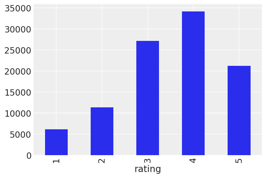
data.rating.describe()
count    100000.000000
mean          3.529860
std           1.125674
min           1.000000
25%           3.000000
50%           4.000000
75%           4.000000
max           5.000000
Name: rating, dtype: float64
这一定是一批不错的电影。从我们上面的探索中,我们知道大多数评分都在 3 到 5 的范围内,并且正面评分比负面评分更常见。让我们看看每部电影的平均值,看看我们这里是否有特别好(或坏)的电影。
movie_means = data.join(movies["movie title"], on="itemid").groupby("movie title").rating.mean()
movie_means[:50].plot(kind="bar", grid=False, figsize=(16, 6), title="Mean ratings for 50 movies");
/Users/severinhatt/miniconda3/envs/pymc-hack/lib/python3.9/site-packages/IPython/core/pylabtools.py:151: UserWarning: constrained_layout not applied because axes sizes collapsed to zero.  Try making figure larger or axes decorations smaller.
  fig.canvas.print_figure(bytes_io, **kw)
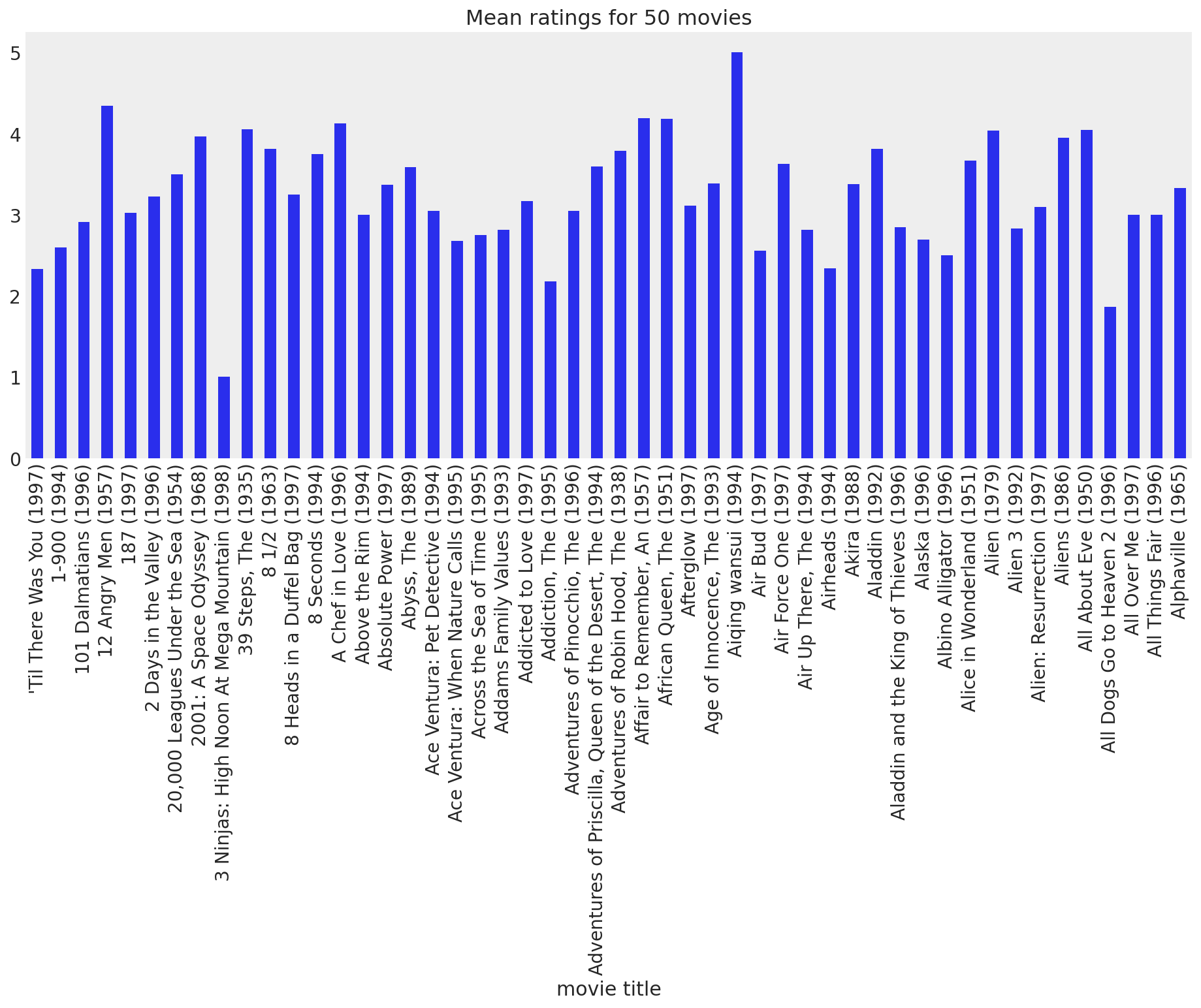
虽然大多数电影通常会收到用户的正面反馈,但肯定有一些电影显得很糟糕。让我们看看最差和最好的电影,只是为了好玩
fig, (ax1, ax2) = plt.subplots(ncols=2, figsize=(16, 4), sharey=True)
movie_means.nlargest(30).plot(kind="bar", ax=ax1, title="Top 30 movies in data set")
movie_means.nsmallest(30).plot(kind="bar", ax=ax2, title="Bottom 30 movies in data set");
/Users/severinhatt/miniconda3/envs/pymc-hack/lib/python3.9/site-packages/IPython/core/pylabtools.py:151: UserWarning: constrained_layout not applied because axes sizes collapsed to zero.  Try making figure larger or axes decorations smaller.
  fig.canvas.print_figure(bytes_io, **kw)
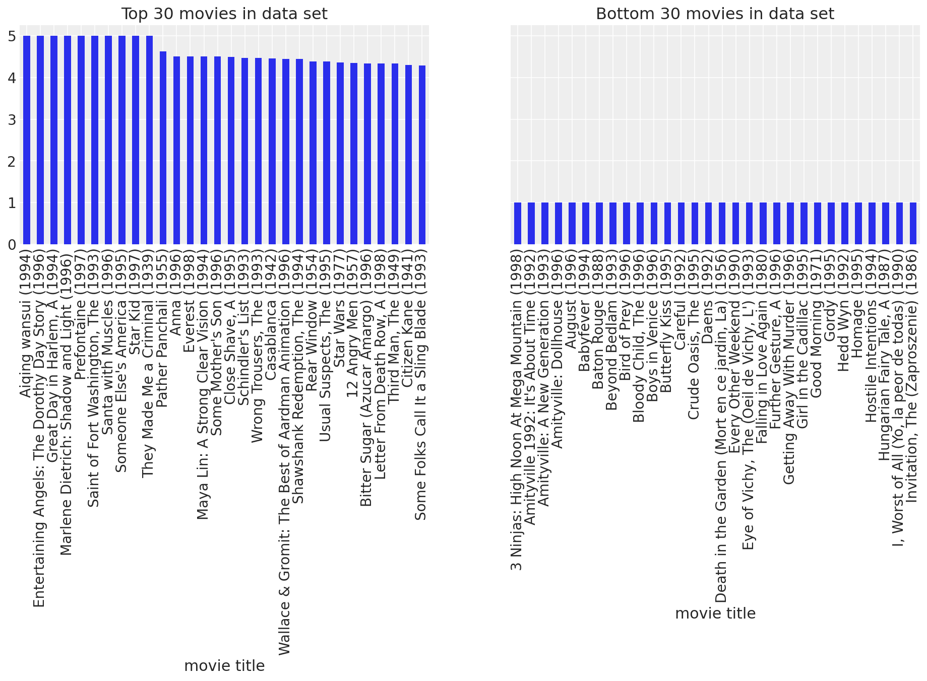
我明白了。我们现在知道电影之间肯定存在受欢迎程度差异。有些电影比其他电影更好,有些电影简直太糟糕了。查看电影平均值使我们能够发现这些总体趋势。也许用户之间也存在类似的趋势。可能有些用户比其他用户更容易被娱乐。让我们来看看。
user_means = data.groupby("userid").rating.mean().sort_values()
_, ax = plt.subplots(figsize=(16, 6))
ax.plot(np.arange(len(user_means)), user_means.values, "k-")

ax.fill_between(np.arange(len(user_means)), user_means.values, alpha=0.3)
ax.set_xticklabels("")
# 1000 labels is nonsensical
ax.set_ylabel("Rating")
ax.set_xlabel(f"{len(user_means)} average ratings per user")
ax.set_ylim(0, 5)
ax.set_xlim(0, len(user_means));
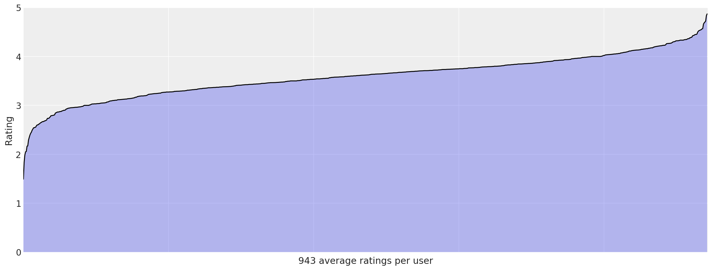
我们在这里看到了更明显的趋势。有些用户几乎对所有内容都给予高度评价,而有些用户(虽然没有那么多)几乎对所有内容都给予负面评价。在考虑用于预测用户对未看过电影的偏好的模型时,这些观察结果将派上用场。
方法#
探索了数据后,我们现在准备深入研究并开始解决问题。我们想预测每个用户会喜欢所有他或她尚未看过的电影的程度。
基线#
每个好的分析都需要一些基线方法来进行比较。如果我们没有定义“好”的参考点,就很难声称我们已经产生了好的结果。我们将定义三种非常简单的基线方法,并使用这些方法找到 RMSE。我们的目标是使用我们产生的任何模型获得更低的 RMSE 分数。
均匀随机基线#
我们的第一个基线非常愚蠢。在我们看到 \(R\) 中缺少值的地方,我们将简单地用在 [1, 5] 范围内均匀随机抽取的数字填充它。我们预计这种方法的效果会差得多。
全局平均基线#
这种方法仅比上一种方法略好。无论我们在哪里缺少值,我们都将用所有观察到的评分的平均值来填充它。
均值平均基线#
现在我们要开始变得更聪明一些了。我们想象有些用户可能很容易被逗乐,并且倾向于对所有电影给予更高的评价。其他用户可能恰恰相反。此外,有些电影可能只是比其他电影更有趣,因此所有用户可能总体上会对某些电影给予比其他电影更高的评价。我们可以在上面电影平均值的图中清楚地看到这一点。我们将尝试通过每个用户和每部电影的评分平均值来捕获这些总体趋势。我们还将结合全局平均值来稍微平滑一下。因此,如果我们看到单元格 \(R_{ij}\) 中缺少值,我们将全局平均值与 \(U_i\) 的平均值和 \(V_j\) 的平均值平均,并使用该值来填充它。
# Create a base class with scaffolding for our 3 baselines.


def split_title(title):
    """Change "BaselineMethod" to "Baseline Method"."""
    words = []
    tmp = [title[0]]
    for c in title[1:]:
        if c.isupper():
            words.append("".join(tmp))
            tmp = [c]
        else:
            tmp.append(c)
    words.append("".join(tmp))
    return " ".join(words)


class Baseline:
    """Calculate baseline predictions."""

    def __init__(self, train_data):
        """Simple heuristic-based transductive learning to fill in missing
        values in data matrix."""
        self.predict(train_data.copy())

    def predict(self, train_data):
        raise NotImplementedError("baseline prediction not implemented for base class")

    def rmse(self, test_data):
        """Calculate root mean squared error for predictions on test data."""
        return rmse(test_data, self.predicted)

    def __str__(self):
        return split_title(self.__class__.__name__)


# Implement the 3 baselines.


class UniformRandomBaseline(Baseline):
    """Fill missing values with uniform random values."""

    def predict(self, train_data):
        nan_mask = np.isnan(train_data)
        masked_train = np.ma.masked_array(train_data, nan_mask)
        pmin, pmax = masked_train.min(), masked_train.max()
        N = nan_mask.sum()
        train_data[nan_mask] = rng.uniform(pmin, pmax, N)
        self.predicted = train_data


class GlobalMeanBaseline(Baseline):
    """Fill in missing values using the global mean."""

    def predict(self, train_data):
        nan_mask = np.isnan(train_data)
        train_data[nan_mask] = train_data[~nan_mask].mean()
        self.predicted = train_data


class MeanOfMeansBaseline(Baseline):
    """Fill in missing values using mean of user/item/global means."""

    def predict(self, train_data):
        nan_mask = np.isnan(train_data)
        masked_train = np.ma.masked_array(train_data, nan_mask)
        global_mean = masked_train.mean()
        user_means = masked_train.mean(axis=1)
        item_means = masked_train.mean(axis=0)
        self.predicted = train_data.copy()
        n, m = train_data.shape
        for i in range(n):
            for j in range(m):
                if np.ma.isMA(item_means[j]):
                    self.predicted[i, j] = np.mean((global_mean, user_means[i]))
                else:
                    self.predicted[i, j] = np.mean((global_mean, user_means[i], item_means[j]))


baseline_methods = {}
baseline_methods["ur"] = UniformRandomBaseline
baseline_methods["gm"] = GlobalMeanBaseline
baseline_methods["mom"] = MeanOfMeansBaseline
num_users = data.userid.unique().shape[0]
num_items = data.itemid.unique().shape[0]
sparsity = 1 - len(data) / (num_users * num_items)
print(f"Users: {num_users}\nMovies: {num_items}\nSparsity: {sparsity}")

dense_data = data.pivot(index="userid", columns="itemid", values="rating").values
Users: 943
Movies: 1682
Sparsity: 0.9369533063577546
概率矩阵分解#
概率矩阵分解 [Mnih and Salakhutdinov, 2008] 是一种概率方法,用于解决采用贝叶斯观点的协同过滤问题。评分 \(R\) 被建模为从高斯分布中抽取的样本。\(R_{ij}\) 的均值是 \(U_i V_j^T\)。精度 \(\alpha\) 是一个固定的参数,它反映了估计的不确定性;正态分布通常根据精度重新参数化,精度是方差的倒数。复杂性通过在 \(U\) 和 \(V\) 上放置零均值球面高斯先验来控制。换句话说,\(U\) 的每一行都是从均值 \(\mu = 0\) 和精度是单位矩阵 \(I\) 的某个倍数的多变量高斯分布中抽取的。这些倍数对于 \(U\) 是 \(\alpha_U\),对于 \(V\) 是 \(\alpha_V\)。因此,我们的模型由下式定义
\(\newcommand\given[1][]{\:#1\vert\:}\)
给定小的精度参数,\(U\) 和 \(V\) 的先验确保我们的潜在变量不会离 0 太远。这防止了学习到过于强的用户偏好和项目因子组成。这通常被称为复杂性控制,其中模型的复杂性在这里通过潜在变量的大小来衡量。像这样控制复杂性有助于防止过拟合,这使得模型能够更好地泛化到未见过的数据。我们还必须为 \(R\) 的正态分布选择合适的 \(\alpha\) 值。因此,挑战变成了为 \(\alpha_U\)、\(\alpha_V\) 和 \(\alpha\) 选择合适的值。这个挑战可以通过 Nowlan 和 Hinton [1992] 讨论的软权重共享方法来解决。但是,为了进行此分析,我们将坚持使用从我们的数据中获得的点估计。
import logging
import time

import pytensor
import scipy as sp

# Enable on-the-fly graph computations, but ignore
# absence of intermediate test values.
pytensor.config.compute_test_value = "ignore"

# Set up logging.
logger = logging.getLogger()
logger.setLevel(logging.INFO)


class PMF:
    """Probabilistic Matrix Factorization model using pymc."""

    def __init__(self, train, dim, alpha=2, std=0.01, bounds=(1, 5)):
        """Build the Probabilistic Matrix Factorization model using pymc.

        :param np.ndarray train: The training data to use for learning the model.
        :param int dim: Dimensionality of the model; number of latent factors.
        :param int alpha: Fixed precision for the likelihood function.
        :param float std: Amount of noise to use for model initialization.
        :param (tuple of int) bounds: (lower, upper) bound of ratings.
            These bounds will simply be used to cap the estimates produced for R.

        """
        self.dim = dim
        self.alpha = alpha
        self.std = np.sqrt(1.0 / alpha)
        self.bounds = bounds
        self.data = train.copy()
        n, m = self.data.shape

        # Perform mean value imputation
        nan_mask = np.isnan(self.data)
        self.data[nan_mask] = self.data[~nan_mask].mean()

        # Low precision reflects uncertainty; prevents overfitting.
        # Set to the mean variance across users and items.
        self.alpha_u = 1 / self.data.var(axis=1).mean()
        self.alpha_v = 1 / self.data.var(axis=0).mean()

        # Specify the model.
        logging.info("building the PMF model")
        with pm.Model(
            coords={
                "users": np.arange(n),
                "movies": np.arange(m),
                "latent_factors": np.arange(dim),
                "obs_id": np.arange(self.data[~nan_mask].shape[0]),
            }
        ) as pmf:
            U = pm.MvNormal(
                "U",
                mu=0,
                tau=self.alpha_u * np.eye(dim),
                dims=("users", "latent_factors"),
                initval=rng.standard_normal(size=(n, dim)) * std,
            )
            V = pm.MvNormal(
                "V",
                mu=0,
                tau=self.alpha_v * np.eye(dim),
                dims=("movies", "latent_factors"),
                initval=rng.standard_normal(size=(m, dim)) * std,
            )
            R = pm.Normal(
                "R",
                mu=(U @ V.T)[~nan_mask],
                tau=self.alpha,
                dims="obs_id",
                observed=self.data[~nan_mask],
            )

        logging.info("done building the PMF model")
        self.model = pmf

    def __str__(self):
        return self.name
我们还需要用于计算 MAP 并在我们的 PMF 模型上执行采样的函数。当观测噪声方差 \(\alpha\) 和先验方差 \(\alpha_U\) 和 \(\alpha_V\) 都保持固定时,最大化对数后验等效于最小化具有二次正则化项的平方误差目标函数之和。
其中 \(\lambda_U = \alpha_U / \alpha\),\(\lambda_V = \alpha_V / \alpha\),并且 \(\|\cdot\|_{Fro}^2\) 表示 Frobenius 范数 [Mnih and Salakhutdinov, 2008]。最小化此目标函数会得到局部最小值,这本质上是最大后验 (MAP) 估计。虽然可以使用快速随机梯度下降程序来找到此 MAP,但我们将使用内置于 pymc 中的实用程序来找到它。特别是,我们将使用 Powell 优化 (scipy.optimize.fmin_powell) 的 find_MAP。找到此 MAP 估计后,我们可以将其用作 MCMC 采样的起点。
由于它是一个相当复杂的模型,我们预计 MAP 估计需要一些时间。因此,让我们在找到它之后保存它。请注意,我们在下面定义了一个用于查找 MAP 的函数,假设它将接收一个包含一些变量的命名空间。然后,我们将该函数附加到 PMF 类,在初始化之后,它将在其中具有这样的命名空间。PMF 类以这种方式分段定义,以便我可以在每段之间说几句话,使其更清晰。
def _find_map(self):
    """Find mode of posterior using L-BFGS-B optimization."""
    tstart = time.time()
    with self.model:
        logging.info("finding PMF MAP using L-BFGS-B optimization...")
        self._map = pm.find_MAP(method="L-BFGS-B")

    elapsed = int(time.time() - tstart)
    logging.info("found PMF MAP in %d seconds" % elapsed)
    return self._map


def _map(self):
    try:
        return self._map
    except:
        return self.find_map()


# Update our class with the new MAP infrastructure.
PMF.find_map = _find_map
PMF.map = property(_map)
所以现在我们的 PMF 类有一个 map property,它将使用 Powell 优化找到,或者从以前的优化中加载。一旦我们有了 MAP,我们就可以将其用作 MCMC 采样器的起点。我们将需要一个采样函数,以便绘制 MCMC 样本来近似 PMF 模型的后验分布。
# Draw MCMC samples.
def _draw_samples(self, **kwargs):
    # kwargs.setdefault("chains", 1)
    with self.model:
        self.trace = pm.sample(**kwargs)


# Update our class with the sampling infrastructure.
PMF.draw_samples = _draw_samples
我们可以像对 MAP 那样定义某种默认的跟踪属性,但这将意味着对 nsamples 和 cores 使用可能毫无意义的值。最好将其保留为对 draw_samples 的非可选调用。最后,我们将需要一个函数来使用我们推断出的 \(U\) 和 \(V\) 值进行预测。对于用户 \(i\) 和电影 \(j\),预测是通过从 \(\mathcal{N}(U_i V_j^T, \alpha)\) 中抽取样本生成的。为了从采样器生成预测,我们为每个采样的 \(U\) 和 \(V\) 生成一个 \(R\) 矩阵,然后我们通过对 \(K\) 个样本求平均值来组合这些矩阵。
我们希望在平均它们以进行诊断之前检查各个 \(R\) 矩阵。因此,我们将在评估期间编写用于平均的代码。下面的函数只是给定 \(U\) 和 \(V\) 以及存储在 PMF 对象中的固定 \(\alpha\) 来绘制一个 \(R\) 矩阵。
def _predict(self, U, V):
    """Estimate R from the given values of U and V."""
    R = np.dot(U, V.T)
    sample_R = rng.normal(R, self.std)
    # bound ratings
    low, high = self.bounds
    sample_R[sample_R < low] = low
    sample_R[sample_R > high] = high
    return sample_R


PMF.predict = _predict
最后要注意的一点:此模型中的点积通常使用 logistic 函数 \(g(x) = 1/(1 + exp(-x))\) 进行约束,该函数将预测值限制在 [0, 1] 范围内。为了方便这种限制,评分也使用 \(t(x) = (x + min) / range\) 映射到 [0, 1] 范围内。PMF 的作者还引入了一个约束版本,该版本在评分较少的用户上表现更好 [Salakhutdinov and Mnih, 2008]。这两种模型通常都是对此处介绍的基本模型的改进。但是,考虑到时间和空间,这里不会实现这些模型。
评估#
指标#
为了了解我们的模型有多有效,我们需要能够评估它们。我们将根据均方根误差 (RMSE) 进行评估,其形式如下
在这种情况下,RMSE 可以被认为是我们的预测与实际用户偏离的标准偏差。
# Define our evaluation function.
def rmse(test_data, predicted):
    """Calculate root mean squared error.
    Ignoring missing values in the test data.
    """
    I = ~np.isnan(test_data)  # indicator for missing values
    N = I.sum()  # number of non-missing values
    sqerror = abs(test_data - predicted) ** 2  # squared error array
    mse = sqerror[I].sum() / N  # mean squared error
    return np.sqrt(mse)  # RMSE
训练数据与测试数据#
我们接下来需要做的是将我们的数据拆分为训练集和测试集。矩阵分解技术使用转导学习而不是归纳学习。因此,我们通过从完整的 \(N \times M\) 数据矩阵中随机抽取单元格样本来生成测试集。在原始数据矩阵的副本中,选作测试样本的值将替换为 nan 值,以生成训练集。由于我们将生成随机拆分,因此我们还要写出生成的训练/测试集。这将使我们能够复制我们的结果。我们希望能够识别哪个拆分是哪个拆分,因此我们将获取为测试选择的索引的哈希值,并使用它来保存数据。
# Define a function for splitting train/test data.
def split_train_test(data, percent_test=0.1):
    """Split the data into train/test sets.
    :param int percent_test: Percentage of data to use for testing. Default 10.
    """
    n, m = data.shape  # # users, # movies
    N = n * m  # # cells in matrix

    # Prepare train/test ndarrays.
    train = data.copy()
    test = np.ones(data.shape) * np.nan

    # Draw random sample of training data to use for testing.
    tosample = np.where(~np.isnan(train))  # ignore nan values in data
    idx_pairs = list(zip(tosample[0], tosample[1]))  # tuples of row/col index pairs

    test_size = int(len(idx_pairs) * percent_test)  # use 10% of data as test set
    train_size = len(idx_pairs) - test_size  # and remainder for training

    indices = np.arange(len(idx_pairs))  # indices of index pairs
    sample = rng.choice(indices, replace=False, size=test_size)

    # Transfer random sample from train set to test set.
    for idx in sample:
        idx_pair = idx_pairs[idx]
        test[idx_pair] = train[idx_pair]  # transfer to test set
        train[idx_pair] = np.nan  # remove from train set

    # Verify everything worked properly
    assert train_size == N - np.isnan(train).sum()
    assert test_size == N - np.isnan(test).sum()

    # Return train set and test set
    return train, test


train, test = split_train_test(dense_data)
结果#
# Let's see the results:
baselines = {}
for name in baseline_methods:
    Method = baseline_methods[name]
    method = Method(train)
    baselines[name] = method.rmse(test)
    print("{} RMSE:\t{:.5f}".format(method, baselines[name]))
Uniform Random Baseline RMSE:	1.68490
Global Mean Baseline RMSE:	1.11492
Mean Of Means Baseline RMSE:	1.00750
正如预期的那样:均匀随机基线是最差的,全局平均基线是次好的,而均值平均方法是我们最好的基线。现在让我们看看 PMF 的表现如何。
# We use a fixed precision for the likelihood.
# This reflects uncertainty in the dot product.
# We choose 2 in the footsteps Salakhutdinov
# Mnihof.
ALPHA = 2

# The dimensionality D; the number of latent factors.
# We can adjust this higher to try to capture more subtle
# characteristics of each movie. However, the higher it is,
# the more expensive our inference procedures will be.
# Specifically, we have D(N + M) latent variables. For our
# Movielens dataset, this means we have D(2625), so for 5
# dimensions, we are sampling 13125 latent variables.
DIM = 10


pmf = PMF(train, DIM, ALPHA, std=0.05)
显示代码单元格输出
INFO:root:building the PMF model
INFO:root:done building the PMF model
使用 MAP 进行预测#
# Find MAP for PMF.
pmf.find_map();
显示代码单元格输出
INFO:root:finding PMF MAP using L-BFGS-B optimization...
INFO:root:found PMF MAP in 5 seconds
非常棒。我们首先要做的是确保我们获得的 MAP 估计是合理的。我们可以通过计算从 \(U\) 和 \(V\) 的 MAP 值获得的预测评分的 RMSE 来做到这一点。首先,我们定义一个函数,用于从 \(U\) 和 \(V\) 生成预测评分 \(R\)。我们通过将所有低于 1 的值设置为 1,将所有高于 5 的值设置为 5,来确保实际评分范围得到执行。最后,我们计算训练集和测试集的 RMSE。我们预计测试 RMSE 会更高。两者之间的差异在一定程度上说明了我们过度拟合的程度。总是会存在一些差异,但是训练集上非常低的 RMSE 和测试集上非常高的 RMSE 绝对是过度拟合的迹象。
def eval_map(pmf_model, train, test):
    U = pmf_model.map["U"]
    V = pmf_model.map["V"]
    # Make predictions and calculate RMSE on train & test sets.
    predictions = pmf_model.predict(U, V)
    train_rmse = rmse(train, predictions)
    test_rmse = rmse(test, predictions)
    overfit = test_rmse - train_rmse

    # Print report.
    print("PMF MAP training RMSE: %.5f" % train_rmse)
    print("PMF MAP testing RMSE:  %.5f" % test_rmse)
    print("Train/test difference: %.5f" % overfit)

    return test_rmse


# Add eval function to PMF class.
PMF.eval_map = eval_map
# Evaluate PMF MAP estimates.
pmf_map_rmse = pmf.eval_map(train, test)
pmf_improvement = baselines["mom"] - pmf_map_rmse
print("PMF MAP Improvement:   %.5f" % pmf_improvement)
PMF MAP training RMSE: 2.63259
PMF MAP testing RMSE:  2.63524
Train/test difference: 0.00265
PMF MAP Improvement:   -1.62774
实际上,我们看到 MAP 估计和均值均值性能之间的性能有所下降。我们还看到训练集和测试集之间的 RMSE 值存在相当大的差异。这表明我们从数据中计算出的 \(\alpha_U\) 和 \(\alpha_V\) 的点估计在控制模型复杂度方面做得不够好。
让我们看看是否可以通过使用 MCMC 抽样逼近后验分布来改进我们的估计。我们将抽取 500 个样本,其中包含 500 个调整样本。
使用 MCMC 的预测#
# Draw MCMC samples.
pmf.draw_samples(draws=500, tune=500)
显示代码单元格输出
Auto-assigning NUTS sampler...
INFO:pymc:Auto-assigning NUTS sampler...
Initializing NUTS using jitter+adapt_diag...
INFO:pymc:Initializing NUTS using jitter+adapt_diag...
/Users/severinhatt/miniconda3/envs/pymc-hack/lib/python3.9/site-packages/pymc/pytensorf.py:1005: UserWarning: The parameter 'updates' of pytensor.function() expects an OrderedDict, got <class 'dict'>. Using a standard dictionary here results in non-deterministic behavior. You should use an OrderedDict if you are using Python 2.7 (collections.OrderedDict for older python), or use a list of (shared, update) pairs. Do not just convert your dictionary to this type before the call as the conversion will still be non-deterministic.
  pytensor_function = pytensor.function(
Multiprocess sampling (4 chains in 4 jobs)
INFO:pymc:Multiprocess sampling (4 chains in 4 jobs)
NUTS: [U, V]
INFO:pymc:NUTS: [U, V]
Sampling 4 chains for 500 tune and 500 draw iterations (2_000 + 2_000 draws total) took 2194 seconds.
INFO:pymc:Sampling 4 chains for 500 tune and 500 draw iterations (2_000 + 2_000 draws total) took 2194 seconds.
The rhat statistic is larger than 1.01 for some parameters. This indicates problems during sampling. See https://arxiv.org/abs/1903.08008 for details
INFO:pymc:The rhat statistic is larger than 1.01 for some parameters. This indicates problems during sampling. See https://arxiv.org/abs/1903.08008 for details
The effective sample size per chain is smaller than 100 for some parameters.  A higher number is needed for reliable rhat and ess computation. See https://arxiv.org/abs/1903.08008 for details
ERROR:pymc:The effective sample size per chain is smaller than 100 for some parameters.  A higher number is needed for reliable rhat and ess computation. See https://arxiv.org/abs/1903.08008 for details
诊断和后验预测检查#
下一步是检查我们应该丢弃多少样本作为预热期。通常,我们会使用迹图来了解采样变量何时开始收敛。在这种情况下,我们有高维样本,因此我们需要找到一种方法来逼近它们。Salakhutdinov 和 Mnih [2008] 提出了一个方法。我们可以计算每个步骤中 \(U\) 和 \(V\) 的 Frobenius 范数,并监测它们的收敛情况。这本质上让我们了解潜在变量的平均幅度何时趋于稳定。\(U\) 和 \(V\) 的 Frobenius 范数的方程如下所示。我们将使用 numpy 的 linalg 包来计算这些范数。
def _norms(pmf_model):
    """Return norms of latent variables at each step in the
    sample trace. These can be used to monitor convergence
    of the sampler.
    """

    norms = dict()
    norms["U"] = xr.apply_ufunc(
        np.linalg.norm,
        pmf_model.trace.posterior["U"],
        input_core_dims=[["users", "latent_factors"]],
        kwargs={"ord": "fro", "axis": (-2, -1)},
    )
    norms["V"] = xr.apply_ufunc(
        np.linalg.norm,
        pmf_model.trace.posterior["V"],
        input_core_dims=[["movies", "latent_factors"]],
        kwargs={"ord": "fro", "axis": (-2, -1)},
    )

    return xr.Dataset(norms)


def _traceplot(pmf_model):
    """Plot Frobenius norms of U and V as a function of sample #."""
    fig, ax = plt.subplots(2, 2, figsize=(12, 7))
    az.plot_trace(pmf_model.norms(), axes=ax)
    ax[0][1].set_title(label=r"$\|U\|_{Fro}^2$ at Each Sample", fontsize=10)
    ax[1][1].set_title(label=r"$\|V\|_{Fro}^2$ at Each Sample", fontsize=10)
    ax[1][1].set_xlabel("Sample Number", fontsize=10)


PMF.norms = _norms
PMF.traceplot = _traceplot
pmf.traceplot()
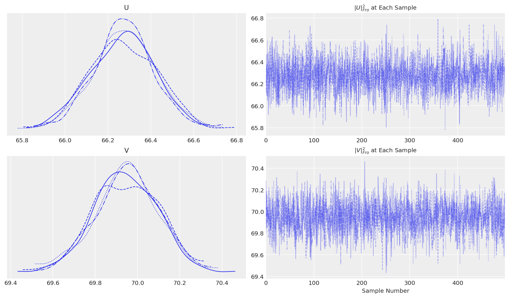
看来我们在大约默认调整后获得了 \(U\) 和 \(V\) 的收敛。在测试收敛性时,我们还希望看到我们正在寻找的特定统计量的收敛性,因为后验的不同特征可能以不同的速率收敛。让我们也做一个 RSME 的迹图。我们将计算训练集和测试集的 RMSE,即使收敛性仅由训练集上的 RMSE 指示。此外,让我们计算训练/测试集上的运行 RMSE,以查看随着我们继续采样,总体性能如何提高或降低。
请注意,这里我们仅从 1 个链中进行采样,这使得诸如 \(\hat{R}\) 之类的收敛统计量变得不可能(我们仍然可以计算 split-rhat,但目的不同)。不采样多个链的原因是 PMF 可能没有唯一的解。因此,在没有约束的情况下,解充其量是对称的,在任何旋转下充其量是相同的,在任何情况下都受标签切换的影响。事实上,如果我们从多个链中进行采样,我们将看到大的 \(\hat{R}\),表明采样器正在探索参数空间不同部分的不同解。
def _running_rmse(pmf_model, test_data, train_data, plot=True):
    """Calculate RMSE for each step of the trace to monitor convergence."""
    results = {"per-step-train": [], "running-train": [], "per-step-test": [], "running-test": []}
    R = np.zeros(test_data.shape)
    for cnt in pmf.trace.posterior.draw.values:
        U = pmf_model.trace.posterior["U"].sel(chain=0, draw=cnt)
        V = pmf_model.trace.posterior["V"].sel(chain=0, draw=cnt)
        sample_R = pmf_model.predict(U, V)
        R += sample_R
        running_R = R / (cnt + 1)
        results["per-step-train"].append(rmse(train_data, sample_R))
        results["running-train"].append(rmse(train_data, running_R))
        results["per-step-test"].append(rmse(test_data, sample_R))
        results["running-test"].append(rmse(test_data, running_R))

    results = pd.DataFrame(results)

    if plot:
        results.plot(
            kind="line",
            grid=False,
            figsize=(15, 7),
            title="Per-step and Running RMSE From Posterior Predictive",
        )

    # Return the final predictions, and the RMSE calculations
    return running_R, results


PMF.running_rmse = _running_rmse
predicted, results = pmf.running_rmse(test, train)
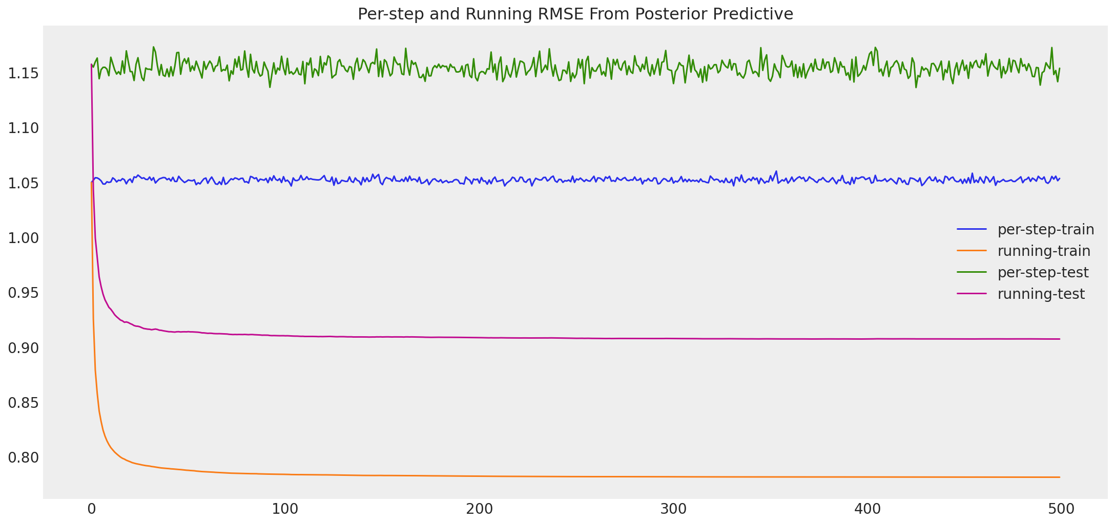
# And our final RMSE?
final_test_rmse = results["running-test"].values[-1]
final_train_rmse = results["running-train"].values[-1]
print("Posterior predictive train RMSE: %.5f" % final_train_rmse)
print("Posterior predictive test RMSE:  %.5f" % final_test_rmse)
print("Train/test difference:           %.5f" % (final_test_rmse - final_train_rmse))
print("Improvement from MAP:            %.5f" % (pmf_map_rmse - final_test_rmse))
print("Improvement from Mean of Means:  %.5f" % (baselines["mom"] - final_test_rmse))
Posterior predictive train RMSE: 0.78127
Posterior predictive test RMSE:  0.90711
Train/test difference:           0.12584
Improvement from MAP:            1.72813
Improvement from Mean of Means:  0.10039
我们在这里得到了一些有趣的结果。正如预期的那样,我们的 MCMC 采样器在训练集上提供了更低的误差。然而,似乎这样做是以过度拟合数据为代价的。与 MAP 相比,这导致测试 RMSE 降低,即使它仍然比我们最好的基线好得多。那么为什么会这样呢?回想一下,我们对精度参数 \(\alpha_U\) 和 \(\alpha_V\) 使用了点估计,并且我们选择了固定的精度 \(\alpha\)。很可能通过这样做,我们以一种将后验偏向训练数据的方式约束了我们的后验。实际上,用户评分和电影评分的方差不太可能等于我们使用的样本方差的均值。此外,最合理的观测精度 \(\alpha\) 也可能不同。
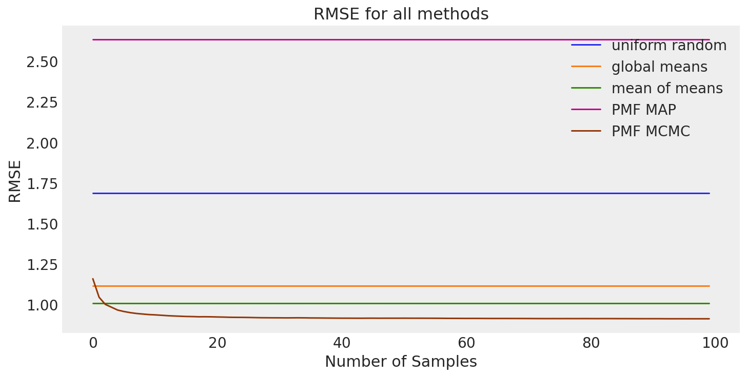
结果总结#
让我们总结一下我们的结果。
size = 100  # RMSE doesn't really change after 100th sample anyway.
all_results = pd.DataFrame(
    {
        "uniform random": np.repeat(baselines["ur"], size),
        "global means": np.repeat(baselines["gm"], size),
        "mean of means": np.repeat(baselines["mom"], size),
        "PMF MAP": np.repeat(pmf_map_rmse, size),
        "PMF MCMC": results["running-test"][:size],
    }
)
fig, ax = plt.subplots(figsize=(10, 5))
all_results.plot(kind="line", grid=False, ax=ax, title="RMSE for all methods")
ax.set_xlabel("Number of Samples")
ax.set_ylabel("RMSE");
总结#
我们着手预测用户对未看过电影的偏好。首先,我们讨论了用户-用户和项目-项目邻域协同过滤方法的直观概念。然后我们形式化了我们的直觉。在对我们的问题背景有了充分的了解之后,我们继续探索 Movielens 数据的子集。在发现一些一般模式之后,我们定义了三种基线方法:均匀随机、全局均值和均值均值。为了超越我们的基线方法,我们使用 pymc 实现了概率矩阵分解 (PMF) 的基本版本。
我们的结果表明,均值均值方法是我们预测任务的最佳基线。正如预期的那样,我们能够使用通过 Powell 优化获得的 PMF MAP 估计显着降低 RMSE。我们说明了一种使用采样变量的 Frobenius 范数来监测具有高维采样空间的 MCMC 采样器收敛性的方法。使用此方法的迹图似乎表明我们的采样器已收敛到后验。使用此后验的结果表明,尝试使用 MCMC 采样改进 MAP 估计实际上过度拟合了训练数据并增加了测试 RMSE。这可能是由于通过固定精度参数 \(\alpha\)、\(\alpha_U\) 和 \(\alpha_V\) 约束后验而引起的。
作为此分析的后续行动,实施 PMF 的逻辑版本和约束版本也会很有趣。我们预计这两种模型都将优于基本 PMF 模型。我们还可以实施 PMF 的完全贝叶斯版本 (BPMF) [Salakhutdinov 和 Mnih,2008],它将超先验置于模型参数上,以自动学习 \(U\) 和 \(V\) 的理想均值和精度参数。这可能会解决我们在此分析中面临的问题。我们预计 BPMF 将通过学习更合适的超参数和参数来改进此处产生的 MAP 估计。有关 pymc 中 BPMF 的基本(但有效!)实现,请参见此 gist。
如果您已经看到这里,那么恭喜您!您现在对如何构建基本的推荐系统有了一些了解。这些相同的想法和方法可以用于许多不同的推荐任务。项目可以是电影、产品、广告、课程,甚至是其他人。任何时候,当您可以构建一个用户-项目矩阵,并在单元格中包含用户偏好时,您都可以使用这些类型的协同过滤算法来预测缺失值。如果您想了解更多关于推荐系统的信息,第一个参考文献是一个很好的起点。
参考文献#
Yehuda Koren、Robert Bell 和 Chris Volinsky。推荐系统的矩阵分解技术。计算机,42(8):30–37, 2009。 doi:10.1109/MC.2009.263。
F. Maxwell Harper 和 Joseph A. Konstan。Movielens 数据集:历史和背景。2016 年 1 月。URL: https://doi.org/10.1145/2827872。
Andriy Mnih 和 Russ R Salakhutdinov。概率矩阵分解。在 J. Platt、D. Koller、Y. Singer 和 S. Roweis 编辑的 神经信息处理系统进展,第 20 卷中。Curran Associates, Inc., 2008。URL: https://proceedings.neurips.cc/paper/2007/file/d7322ed717dedf1eb4e6e52a37ea7bcd-Paper.pdf。
Steven J Nowlan 和 Geoffrey E Hinton。通过软权重共享简化神经网络。神经计算,4(4):473–493, 1992。
Ruslan Salakhutdinov 和 Andriy Mnih。使用马尔可夫链蒙特卡洛的贝叶斯概率矩阵分解。在第 25 届国际机器学习会议论文集,第 25 卷,880–887 页。2008 年。
Ken Goldberg、Theresa Roeder 和 Chris Perkins。Eigentaste:一种恒定时间协同过滤算法。信息检索,4:133–151, 2001。
水印#
%load_ext watermark
%watermark -n -u -v -iv -w -p pytensor,aeppl,xarray
Last updated: Mon Jun 13 2022

Python implementation: CPython
Python version       : 3.9.7
IPython version      : 8.4.0

pytensor: 2.5.1
aeppl : 0.0.27
xarray: 2022.3.0

pandas    : 1.4.2
pymc      : 4.0.0b6
arviz     : 0.12.1
scipy     : 1.7.3
matplotlib: 3.5.2
logging   : 0.5.1.2
pytensor    : 2.5.1
numpy     : 1.22.4
xarray    : 2022.3.0

Watermark: 2.3.1
许可声明#
本示例库中的所有笔记本均根据 MIT 许可证 提供,该许可证允许修改和再分发以用于任何用途,前提是保留版权和许可声明。
引用 PyMC 示例#
要引用此笔记本,请使用 Zenodo 为 pymc-examples 存储库提供的 DOI。
重要提示
许多笔记本都改编自其他来源:博客、书籍等。在这种情况下,您也应该引用原始来源。
另请记住引用您的代码使用的相关库。
这是一个 bibtex 中的引用模板
@incollection{citekey,
  author    = "<notebook authors, see above>",
  title     = "<notebook title>",
  editor    = "PyMC Team",
  booktitle = "PyMC examples",
  doi       = "10.5281/zenodo.5654871"
}
渲染后可能看起来像