高尔夫推杆的模型构建和扩展

这使用了 Andrew Gelman 在 Stan 中编写的案例研究，并与之密切相关。其中包含一些新的可视化效果，并且我们避免使用非正常先验，但非常感谢他和 Stan 团队出色的案例研究和软件。

我们使用了 “Statistics: A Bayesian Perspective” 中的数据集 [Berry, 1996]。该数据集描述了职业高尔夫球手从多个距离推杆的结果，并且数据量很小，我们可以直接打印和加载它，而无需进行任何特殊的 csv 读取。

注意

此 notebook 使用的库不是 PyMC 依赖项，因此需要专门安装才能运行此 notebook。打开下面的下拉菜单以获取更多指导。

额外的依赖项安装说明

为了运行此 notebook（本地或在 binder 上），您不仅需要安装所有可选依赖项的 PyMC 工作环境，还需要安装一些额外的依赖项。有关安装 PyMC 本身的建议，请参阅 安装

您可以使用首选的软件包管理器安装这些依赖项，我们以下面的 pip 和 conda 命令为例。

$ pip install

请注意，如果您想（或需要）从 notebook 内部而不是命令行安装软件包，则可以通过运行 pip 命令的变体来安装软件包

import sys

!{sys.executable} -m pip install

您不应运行 !pip install，因为它可能会将软件包安装在不同的环境中，即使已安装，也无法从 Jupyter notebook 中访问。

另一种选择是使用 conda

$ conda install

当使用 conda 安装科学 python 软件包时，我们建议使用 conda forge

import io

import arviz as az
import matplotlib.pyplot as plt
import numpy as np
import pandas as pd
import pymc as pm
import pytensor.tensor as pt
import scipy
import scipy.stats as st
import xarray as xr

from xarray_einstats.stats import XrContinuousRV

RANDOM_SEED = 8927
az.style.use("arviz-darkgrid")

# golf putting data from berry (1996)
golf_data = """distance tries successes
2 1443 1346
3 694 577
4 455 337
5 353 208
6 272 149
7 256 136
8 240 111
9 217 69
10 200 67
11 237 75
12 202 52
13 192 46
14 174 54
15 167 28
16 201 27
17 195 31
18 191 33
19 147 20
20 152 24"""


golf_data = pd.read_csv(io.StringIO(golf_data), sep=" ", dtype={"distance": "float"})

BALL_RADIUS = (1.68 / 2) / 12
CUP_RADIUS = (4.25 / 2) / 12

我们开始绘制数据以更好地了解其外观。隐藏的单元格包含绘图代码

显示代码单元格源 隐藏代码单元格源

def plot_golf_data(golf_data, ax=None, color="C0"):
    """Utility function to standardize a pretty plotting of the golf data."""
    if ax is None:
        _, ax = plt.subplots()
    bg_color = ax.get_facecolor()
    rv = st.beta(golf_data.successes, golf_data.tries - golf_data.successes)
    ax.vlines(golf_data.distance, *rv.interval(0.68), label=None, color=color)
    ax.plot(
        golf_data.distance,
        golf_data.successes / golf_data.tries,
        "o",
        mec=color,
        mfc=bg_color,
        label=None,
    )

    ax.set_xlabel("Distance from hole")
    ax.set_ylabel("Percent of putts made")
    ax.set_ylim(bottom=0, top=1)

    ax.set_xlim(left=0)
    ax.grid(True, axis="y", alpha=0.7)
    return ax

ax = plot_golf_data(golf_data)
ax.set_title("Overview of data from Berry (1996)");

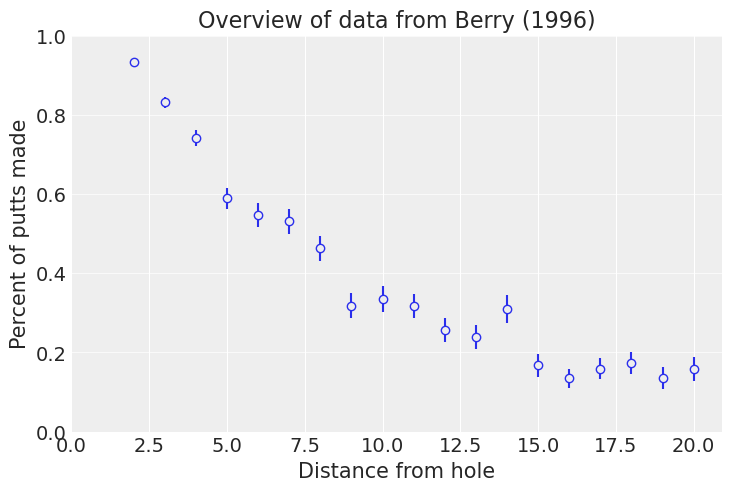
绘制后，我们看到通常高尔夫球手从更远的地方击球的准确性较低。请注意，此数据是预先聚合的：我们或许可以使用更精细的逐杆数据进行更有趣的工作。此数据集似乎已按英尺四舍五入。

我们可能会考虑使用此数据进行预测：将曲线拟合到此数据将使我们能够对中间距离做出合理的猜测，并且可能推断到更远的距离。

逻辑回归模型

首先，我们将拟合传统的逻辑回归-二项式模型。我们直接对成功次数进行建模，使用

\[\begin{split} a, b \sim \mathcal{N}(0, 1) \\ p(\text{成功}) = \operatorname{logit}^{-1}(a \cdot \text{距离} + b) \\ \text{成功次数} \sim \operatorname{Binomial}(\text{尝试次数}, p(\text{成功})) \end{split}\]

以下是如何在 PyMC 中编写该模型。我们在模型变量中使用下划线后缀，以避免污染命名空间。我们还使用 pymc.MutableData，以便稍后在我们处理较新的数据集时可以交换数据。

with pm.Model() as logit_model:
    distance_ = pm.MutableData("distance", golf_data["distance"], dims="obs_id")
    tries_ = pm.MutableData("tries", golf_data["tries"], dims="obs_id")
    successes_ = pm.MutableData("successes", golf_data["successes"], dims="obs_id")

    a_ = pm.Normal("a")
    b_ = pm.Normal("b")

    pm.Binomial(
        "success",
        n=tries_,
        p=pm.math.invlogit(a_ * distance_ + b_),
        observed=successes_,
        dims="obs_id",
    )


pm.model_to_graphviz(logit_model)

我们有一些直觉，即 \(a\) 应该是负数，并且 \(b\) 应该是正数（因为当 \(\text{距离} = 0\) 时，我们期望几乎 100% 的推杆都能成功）。但是，我们没有将此放入模型中。我们将其用作基线，并且不妨等待看看是否需要添加更强的先验。

with logit_model:
    logit_trace = pm.sample(1000, tune=1000, target_accept=0.9)

az.summary(logit_trace)

100.00% [8000/8000 00:00<00:00 采样 4 条链，0 个发散]

Sampling 4 chains for 1_000 tune and 1_000 draw iterations (4_000 + 4_000 draws total) took 1 seconds.

	均值	标准差	hdi_3%	hdi_97%	mcse_mean	mcse_sd	ess_bulk	ess_tail	r_hat
a	-0.255	0.007	-0.268	-0.243	0.000	0.000	880.0	1256.0	1.0
b	2.223	0.057	2.114	2.324	0.002	0.001	931.0	1259.0	1.0

我们看到 \(a\) 和 \(b\) 具有我们预期的符号。采样器没有发出任何不良警告。查看摘要，有效样本数是合理的，并且 rhat 接近 1。这是一个小型模型，因此我们没有过于仔细地检查拟合度。

我们绘制了 \(p(\text{成功})\) 的 50 个后验抽样以及期望值。此外，我们从后验预测中抽取 500 个点进行绘制

# Draw posterior predictive samples
with logit_model:
    logit_trace.extend(pm.sample_posterior_predictive(logit_trace))

# hard to plot more than 400 sensibly
logit_post = az.extract(logit_trace, num_samples=400)
logit_ppc = az.extract(logit_trace, group="posterior_predictive", num_samples=400)
const_data = logit_trace["constant_data"]

logit_ppc_success = logit_ppc["success"] / const_data["tries"]

# Plotting
ax = plot_golf_data(golf_data)
t_ary = np.linspace(CUP_RADIUS - BALL_RADIUS, golf_data.distance.max(), 200)
t = xr.DataArray(t_ary, coords=[("distance", t_ary)])
logit_post["expit"] = scipy.special.expit(logit_post["a"] * t + logit_post["b"])

ax.plot(
    t,
    logit_post["expit"].T,
    lw=1,
    color="C1",
    alpha=0.5,
)

ax.plot(t, logit_post["expit"].mean(dim="sample"), color="C2")

ax.plot(golf_data.distance, logit_ppc_success, "k.", alpha=0.01)
ax.set_title("Logit mean and posterior predictive");

100.00% [4000/4000 00:00<00:00]

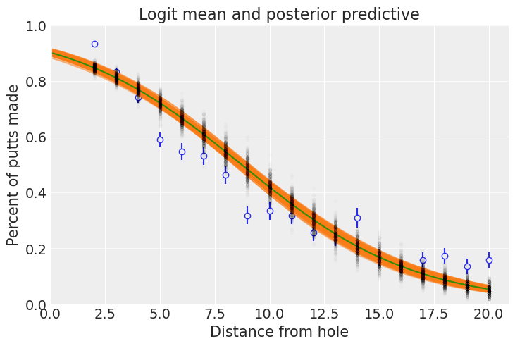
拟合效果还可以，但不是很好！对于基线来说，这是一个好的开始，并且可以让我们回答曲线拟合类型的问题。我们可能不太信任超出数据末尾的太多外推，特别是考虑到曲线与最后四个值拟合得不太好。例如，预计 50 英尺的推杆成功的概率为

prob_at_50 = scipy.special.expit(logit_post["a"] * 50 + logit_post["b"]).mean(dim="sample").item()
print(f"{100 * prob_at_50:.5f}%")

0.00283%

由此得出的教训是

\[ \mathbb{E}[f(\theta)] \ne f(\mathbb{E}[\theta]). \]

这出现在这里，在使用

# Right!
scipy.special.expit(logit_trace.posterior["a"] * 50 + logit_trace.posterior["b"]).mean(dim="sample")

而不是

# Wrong!
scipy.special.expit(logit_trace.posterior["a"].mean(dim="sample") * 50 + logit_trace.posterior["b"].mean(dim="sample"))

来计算我们在 50 英尺处的期望值。

基于几何的模型

作为对该数据建模的第二次尝试，为了提高拟合度和增加对外推的信心，我们考虑情况的几何形状。我们假设职业高尔夫球手可以在某个方向击球，但会存在一些小的（？）误差。具体来说，球实际行进的角度呈正态分布在 0 附近，方差是我们尝试学习的。

然后，当角度误差足够小以至于球仍然击中球杯时，球就会入洞。这在直觉上很不错！较远的推杆允许的角度误差较小，因此成功率低于较短的推杆。

我跳过了推导在给定精度方差和到球洞的距离的情况下推杆成功的概率，但这对于几何学来说是一个有趣的练习，结果证明是

\[ p(\text{成功} | \sigma_{\text{角度}}, \text{距离}) = 2 \Phi\left( \frac{ \arcsin \left((R - r) / \text{距离}\right)}{\sigma_{\text{角度}}}\right), \]

其中 \(\Phi\) 是正态累积密度函数，\(R\) 是球杯的半径（结果是 2.125 英寸），\(r\) 是高尔夫球的半径（大约 0.84 英寸）。

为了了解此模型，让我们看一下 \(\sigma_{\text{角度}}\) 的一些手动绘制的值。

def forward_angle_model(variances_of_shot, t):
    norm_dist = XrContinuousRV(st.norm, 0, variances_of_shot)
    return 2 * norm_dist.cdf(np.arcsin((CUP_RADIUS - BALL_RADIUS) / t)) - 1

_, ax = plt.subplots()
var_shot_ary = [0.01, 0.02, 0.05, 0.1, 0.2, 1]
var_shot_plot = xr.DataArray(var_shot_ary, coords=[("variance", var_shot_ary)])

forward_angle_model(var_shot_plot, t).plot.line(hue="variance")

plot_golf_data(golf_data, ax=ax)
ax.set_title("Model prediction for selected amounts of variance");

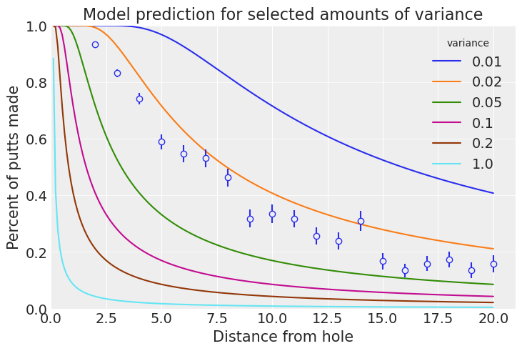
这看起来像是一种很有前景的方法！0.02 弧度的方差看起来会接近正确的答案。该模型还预测，从 0 英尺推杆都会入洞，这是一个不错的副作用。我们可能会考虑高尔夫球手是否对称地错过推杆。对于右手推杆和左手推杆来说，他们的击球可能存在不同的偏差，这是合理的。

拟合模型

PyMC 实现了 \(\Phi\)，但它非常隐藏 (pm.distributions.dist_math.normal_lcdf)，无论如何，我们自己实现它也是值得的，使用与误差函数的恒等式。

def phi(x):
    """Calculates the standard normal cumulative distribution function."""
    return 0.5 + 0.5 * pt.erf(x / pt.sqrt(2.0))


with pm.Model() as angle_model:
    distance_ = pm.MutableData("distance", golf_data["distance"], dims="obs_id")
    tries_ = pm.MutableData("tries", golf_data["tries"], dims="obs_id")
    successes_ = pm.MutableData("successes", golf_data["successes"], dims="obs_id")

    variance_of_shot = pm.HalfNormal("variance_of_shot")
    p_goes_in = pm.Deterministic(
        "p_goes_in",
        2 * phi(pt.arcsin((CUP_RADIUS - BALL_RADIUS) / distance_) / variance_of_shot) - 1,
        dims="obs_id",
    )
    success = pm.Binomial("success", n=tries_, p=p_goes_in, observed=successes_, dims="obs_id")


pm.model_to_graphviz(angle_model)

先验预测检查

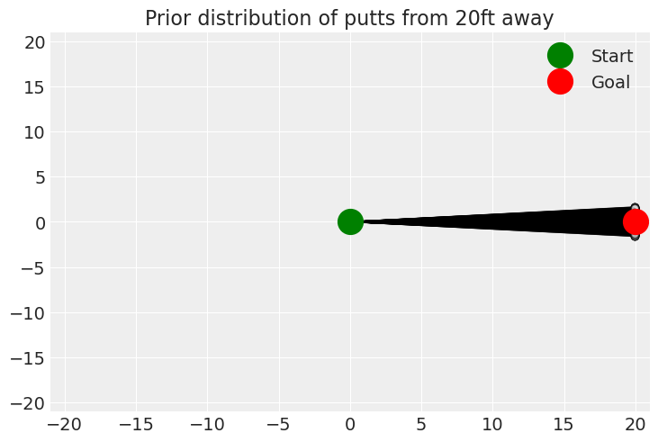
我们经常希望从先验中采样，特别是当我们对观测结果的外观有一些想法，但对先验参数没有太多直觉时。我们这里有一个基于角度的模型，但是如果给定角度的方差，它如何影响击球的准确性可能不直观。让我们检查一下！

有时，自定义可视化或仪表板对于先验预测检查很有用。在这里，我们绘制了 20 英尺外推杆的先验分布。

with angle_model:
    angle_trace = pm.sample_prior_predictive(500)

angle_prior = angle_trace.prior.squeeze()

angle_of_shot = XrContinuousRV(st.norm, 0, angle_prior["variance_of_shot"]).rvs(
    random_state=RANDOM_SEED
)  # radians
distance = 20  # feet

end_positions = xr.Dataset(
    {"endx": distance * np.cos(angle_of_shot), "endy": distance * np.sin(angle_of_shot)}
)

fig, ax = plt.subplots()
for draw in end_positions["draw"]:
    end = end_positions.sel(draw=draw)
    ax.plot([0, end["endx"]], [0, end["endy"]], "k-o", lw=1, mfc="w", alpha=0.5)
ax.plot(0, 0, "go", label="Start", mfc="g", ms=20)
ax.plot(distance, 0, "ro", label="Goal", mfc="r", ms=20)

ax.set_title(f"Prior distribution of putts from {distance}ft away")

ax.legend();

Sampling: [success, variance_of_shot]

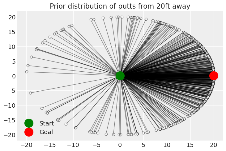
这有点有趣！最明显的是，将球推回应该不太常见。这也让我们担心我们正在使用正态分布来建模角度。冯·米塞斯分布可能在此处适用。此外，高尔夫球手需要站在某个地方，因此可能需要向冯·米塞斯分布添加一些边界。但是，我们将发现此模型可以很好地从数据中学习，并且这些添加不是必需的。

with angle_model:
    angle_trace.extend(pm.sample(1000, tune=1000, target_accept=0.85))

angle_post = az.extract(angle_trace)

100.00% [8000/8000 00:00<00:00 采样 4 条链，0 个发散]

Sampling 4 chains for 1_000 tune and 1_000 draw iterations (4_000 + 4_000 draws total) took 1 seconds.

ax = plot_golf_data(golf_data)

angle_post["expit"] = forward_angle_model(angle_post["variance_of_shot"], t)

ax.plot(
    t,
    angle_post["expit"][:, ::100],
    lw=1,
    color="C1",
    alpha=0.1,
)

ax.plot(
    t,
    angle_post["expit"].mean(dim="sample"),
    label="Geometry-based model",
)

ax.plot(
    t,
    logit_post["expit"].mean(dim="sample"),
    label="Logit-binomial model",
)
ax.set_title("Comparing the fit of geometry-based and logit-binomial model")
ax.legend();

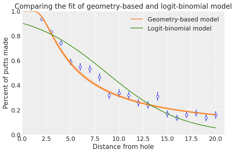
这个新模型似乎拟合得更好，并且通过对情况的几何形状进行建模，我们可能对外推数据更有信心。该模型表明，50 英尺的推杆入洞的机会更高

angle_prob_at_50 = forward_angle_model(angle_post["variance_of_shot"], np.array([50]))
print(f"{100 * angle_prob_at_50.mean().item():.2f}% vs {100 * prob_at_50:.5f}%")

6.40% vs 0.00283%

我们还可以重新创建我们的先验预测图，这让我们对先验没有导致后验分布中不合理的情况充满信心：角度的方差非常小！

angle_of_shot = XrContinuousRV(st.norm, 0, angle_post["variance_of_shot"]).rvs(
    random_state=RANDOM_SEED
)  # radians
distance = 20  # feet

end_positions = xr.Dataset(
    {"endx": distance * np.cos(angle_of_shot.data), "endy": distance * np.sin(angle_of_shot.data)}
)

fig, ax = plt.subplots()
for x, y in zip(end_positions.endx, end_positions.endy):
    ax.plot([0, x], [0, y], "k-o", lw=1, mfc="w", alpha=0.5)
ax.plot(0, 0, "go", label="Start", mfc="g", ms=20)
ax.plot(distance, 0, "ro", label="Goal", mfc="r", ms=20)

ax.set_title(f"Prior distribution of putts from {distance}ft away")
ax.set_xlim(-21, 21)
ax.set_ylim(-21, 21)
ax.legend();

新数据！

马克·布罗迪使用了关于推杆的新汇总数据来拟合新模型。我们将使用这个新数据来改进我们的模型

#  golf putting data from Broadie (2018)
new_golf_data = """distance tries successes
0.28 45198 45183
0.97 183020 182899
1.93 169503 168594
2.92 113094 108953
3.93 73855 64740
4.94 53659 41106
5.94 42991 28205
6.95 37050 21334
7.95 33275 16615
8.95 30836 13503
9.95 28637 11060
10.95 26239 9032
11.95 24636 7687
12.95 22876 6432
14.43 41267 9813
16.43 35712 7196
18.44 31573 5290
20.44 28280 4086
21.95 13238 1642
24.39 46570 4767
28.40 38422 2980
32.39 31641 1996
36.39 25604 1327
40.37 20366 834
44.38 15977 559
48.37 11770 311
52.36 8708 231
57.25 8878 204
63.23 5492 103
69.18 3087 35
75.19 1742 24"""

new_golf_data = pd.read_csv(io.StringIO(new_golf_data), sep=" ")

ax = plot_golf_data(new_golf_data)
plot_golf_data(golf_data, ax=ax, color="C1")

t_ary = np.linspace(CUP_RADIUS - BALL_RADIUS, new_golf_data.distance.max(), 200)
t = xr.DataArray(t_ary, coords=[("distance", t_ary)])

ax.plot(
    t, forward_angle_model(angle_trace.posterior["variance_of_shot"], t).mean(("chain", "draw"))
)
ax.set_title("Comparing the new data set to the old data set, and\nconsidering the old model fit");

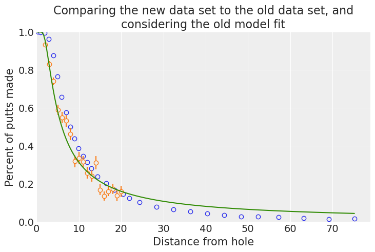
这个新数据集代表的推杆尝试次数大约是旧数据的 200 倍，并且包括高达 75 英尺的推杆，而旧数据集中只有 20 英尺。此外，新数据似乎代表了与旧数据不同的人群：虽然两者具有不同的箱子，但新数据表明大多数数据的成功率更高。这可能是由于收集数据的方法不同，或者是高尔夫球手在过去几年中有所进步。

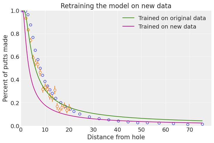
在新数据上拟合模型

由于我们认为这可能是两个不同的人群，最简单的解决方案是重新拟合我们的模型。但这比早期更糟糕：存在发散，并且运行时间更长。这可能表明模型存在问题：安德鲁·格尔曼称之为“统计计算的民间定理”。

with angle_model:
    pm.set_data(
        {
            "distance": new_golf_data["distance"],
            "tries": new_golf_data["tries"],
            "successes": new_golf_data["successes"],
        }
    )
    new_angle_trace = pm.sample(1000, tune=1500)

100.00% [10000/10000 00:14<00:00 采样 4 条链，2,003 个发散]

Sampling 4 chains for 1_500 tune and 1_000 draw iterations (6_000 + 4_000 draws total) took 15 seconds.

注意

正如您将在下面的图中看到的那样，此模型对新数据的拟合非常糟糕。在这种情况下，所有发散和收敛警告除了使用实际上可以解释数据的不同模型之外，别无他法。

ax = plot_golf_data(new_golf_data)
plot_golf_data(golf_data, ax=ax, color="C1")

new_angle_post = az.extract(new_angle_trace)
ax.plot(
    t,
    forward_angle_model(angle_post["variance_of_shot"], t).mean(dim="sample"),
    label="Trained on original data",
)
ax.plot(
    t,
    forward_angle_model(new_angle_post["variance_of_shot"], t).mean(dim="sample"),
    label="Trained on new data",
)
ax.set_title("Retraining the model on new data")
ax.legend();

结合到球洞距离的模型

我们可能会假设，除了朝正确的方向推杆外，高尔夫球手可能还需要击中正确的距离。具体来说，我们假设

1. 如果推杆短了或超过球洞 3 英尺以上，则不会入洞。

2. 高尔夫球手的目标是超过球洞 1 英尺

3. 球行进的距离 \(u\) 根据以下分布：

   \[ u \sim \mathcal{N}\left(1 + \text{距离}, \sigma_{\text{距离}} (1 + \text{距离})\right), \]
   我们将从中学习 \(\sigma_{\text{距离}}\)。

同样，这是一个几何和代数问题，可以计算出球从任何给定距离入洞的概率

\[ P(\text{良好距离}) = P(\text{距离} < u < \text{距离} + 3) \]

它使用 phi，即我们之前实现的累积正态密度函数。

OVERSHOT = 1.0
DISTANCE_TOLERANCE = 3.0


with pm.Model() as distance_angle_model:
    distance_ = pm.MutableData("distance", new_golf_data["distance"], dims="obs_id")
    tries_ = pm.MutableData("tries", new_golf_data["tries"], dims="obs_id")
    successes_ = pm.MutableData("successes", new_golf_data["successes"], dims="obs_id")

    variance_of_shot = pm.HalfNormal("variance_of_shot")
    variance_of_distance = pm.HalfNormal("variance_of_distance")
    p_good_angle = pm.Deterministic(
        "p_good_angle",
        2 * phi(pt.arcsin((CUP_RADIUS - BALL_RADIUS) / distance_) / variance_of_shot) - 1,
        dims="obs_id",
    )
    p_good_distance = pm.Deterministic(
        "p_good_distance",
        phi((DISTANCE_TOLERANCE - OVERSHOT) / ((distance_ + OVERSHOT) * variance_of_distance))
        - phi(-OVERSHOT / ((distance_ + OVERSHOT) * variance_of_distance)),
        dims="obs_id",
    )

    success = pm.Binomial(
        "success", n=tries_, p=p_good_angle * p_good_distance, observed=successes_, dims="obs_id"
    )


pm.model_to_graphviz(distance_angle_model)

此模型仍然只有 2 个维度要拟合。我们可能会考虑检查 OVERSHOT 和 DISTANCE_TOLERANCE。检查第一个可能需要致电当地的高尔夫球场，而第二个可能需要去果岭并花费一些时间进行实验。我们还可能考虑添加一些显式相关性：角度控制较少可能对应于距离控制较少，或者较远的推杆会导致角度的方差更大，这是合理的。

拟合距离角度模型

with distance_angle_model:
    distance_angle_trace = pm.sample(1000, tune=1000, target_accept=0.85)

100.00% [8000/8000 00:03<00:00 采样 4 条链，0 个发散]

Sampling 4 chains for 1_000 tune and 1_000 draw iterations (4_000 + 4_000 draws total) took 4 seconds.

def forward_distance_angle_model(variance_of_shot, variance_of_distance, t):
    rv = XrContinuousRV(st.norm, 0, 1)
    angle_prob = 2 * rv.cdf(np.arcsin((CUP_RADIUS - BALL_RADIUS) / t) / variance_of_shot) - 1

    distance_prob_one = rv.cdf(
        (DISTANCE_TOLERANCE - OVERSHOT) / ((t + OVERSHOT) * variance_of_distance)
    )
    distance_prob_two = rv.cdf(-OVERSHOT / ((t + OVERSHOT) * variance_of_distance))
    distance_prob = distance_prob_one - distance_prob_two

    return angle_prob * distance_prob


ax = plot_golf_data(new_golf_data)

distance_angle_post = az.extract(distance_angle_trace)

ax.plot(
    t,
    forward_angle_model(new_angle_post["variance_of_shot"], t).mean(dim="sample"),
    label="Just angle",
)
ax.plot(
    t,
    forward_distance_angle_model(
        distance_angle_post["variance_of_shot"],
        distance_angle_post["variance_of_distance"],
        t,
    ).mean(dim="sample"),
    label="Distance and angle",
)

ax.set_title("Comparing fits of models on new data")
ax.legend();

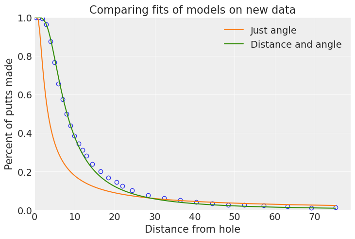
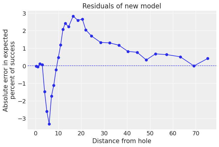
与旧模型相比，这个新模型看起来更好，并且拟合速度更快，采样问题更少。10 到 40 英尺之间存在一些不匹配，但总体上看起来不错。我们可以通过获取后验预测样本并查看残差来得出相同的结论。在这里，我们看到拟合是由前 4 个箱子驱动的，这些箱子包含约 40% 的数据。

with distance_angle_model:
    pm.sample_posterior_predictive(distance_angle_trace, extend_inferencedata=True)

const_data = distance_angle_trace.constant_data
pp = distance_angle_trace.posterior_predictive
residuals = 100 * ((const_data["successes"] - pp["success"]) / const_data["tries"]).mean(
    ("chain", "draw")
)

fig, ax = plt.subplots()

ax.plot(new_golf_data.distance, residuals, "o-")
ax.axhline(y=0, linestyle="dashed", linewidth=1)
ax.set_xlabel("Distance from hole")
ax.set_ylabel("Absolute error in expected\npercent of success")

ax.set_title("Residuals of new model");

100.00% [4000/4000 00:00<00:00]

一个新模型

此时停止是合理的，但是如果我们想在所有地方改进拟合，我们可能需要从 Binomial 中选择不同的似然性，后者非常关心那些具有许多观测值的点。我们可以做的一件事是为每个数据点添加一些独立的额外误差。我们可以通过几种方式做到这一点

1. Binomial 分布通常由观测次数 \(n\) 和单个成功的概率 \(p\) 参数化。我们可以改为通过均值 (\(np\)) 和方差 (\(np(1-p)\)) 对其进行参数化，并将独立于 \(n\) 的误差添加到似然性中。

2. 使用 BetaBinomial 分布，尽管那里的误差仍然（大致）与观测次数成正比

3. 用成功的概率的正态分布来近似二项式。这实际上等同于第一种方法，但不需要自定义分布。请注意，我们将使用 \(p\) 作为均值，并将 \(p(1-p) / n\) 作为方差。一旦我们添加一些离散度 \(\epsilon\)，方差变为 \(p(1-p)/n + \epsilon\)。

我们遵循 Stan 案例研究中的方法 3，并将 1 作为练习留给读者。

with pm.Model() as disp_distance_angle_model:
    distance_ = pm.MutableData("distance", new_golf_data["distance"], dims="obs_id")
    tries_ = pm.MutableData("tries", new_golf_data["tries"], dims="obs_id")
    successes_ = pm.MutableData("successes", new_golf_data["successes"], dims="obs_id")
    obs_prop_ = pm.MutableData(
        "obs_prop", new_golf_data["successes"] / new_golf_data["tries"], dims="obs_id"
    )

    variance_of_shot = pm.HalfNormal("variance_of_shot")
    variance_of_distance = pm.HalfNormal("variance_of_distance")
    dispersion = pm.HalfNormal("dispersion")

    p_good_angle = pm.Deterministic(
        "p_good_angle",
        2 * phi(pt.arcsin((CUP_RADIUS - BALL_RADIUS) / distance_) / variance_of_shot) - 1,
        dims="obs_id",
    )
    p_good_distance = pm.Deterministic(
        "p_good_distance",
        phi((DISTANCE_TOLERANCE - OVERSHOT) / ((distance_ + OVERSHOT) * variance_of_distance))
        - phi(-OVERSHOT / ((distance_ + OVERSHOT) * variance_of_distance)),
        dims="obs_id",
    )

    p = p_good_angle * p_good_distance
    p_success = pm.Normal(
        "p_success",
        mu=p,
        sigma=pt.sqrt(((p * (1 - p)) / tries_) + dispersion**2),
        observed=obs_prop_,  # successes_ / tries_
        dims="obs_id",
    )


pm.model_to_graphviz(disp_distance_angle_model)

with disp_distance_angle_model:
    disp_distance_angle_trace = pm.sample(1000, tune=1000)
    pm.sample_posterior_predictive(disp_distance_angle_trace, extend_inferencedata=True)

100.00% [4000/4000 00:00<00:00]

ax = plot_golf_data(new_golf_data, ax=None)

disp_distance_angle_post = az.extract(disp_distance_angle_trace)

ax.plot(
    t,
    forward_distance_angle_model(
        distance_angle_post["variance_of_shot"],
        distance_angle_post["variance_of_distance"],
        t,
    ).mean(dim="sample"),
    label="Distance and angle",
)
ax.plot(
    t,
    forward_distance_angle_model(
        disp_distance_angle_post["variance_of_shot"],
        disp_distance_angle_post["variance_of_distance"],
        t,
    ).mean(dim="sample"),
    label="Dispersed model",
)
ax.set_title("Comparing dispersed model with binomial distance/angle model")
ax.legend();

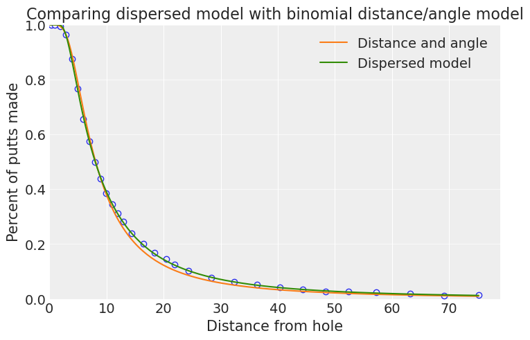
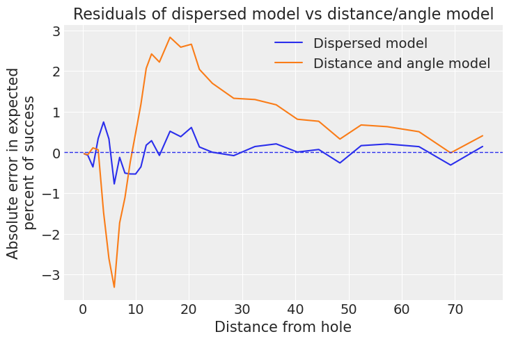
这个新模型在 10 到 30 英尺之间做得更好，正如我们也可以使用残差图看到的那样 - 请注意，对于非常短的推杆，此模型的效果稍差

const_data = distance_angle_trace.constant_data
old_pp = az.extract(distance_angle_trace, group="posterior_predictive")
old_residuals = 100 * ((const_data["successes"] - old_pp["success"]) / const_data["tries"]).mean(
    dim="sample"
)

pp = az.extract(disp_distance_angle_trace, group="posterior_predictive")
residuals = 100 * (const_data["successes"] / const_data["tries"] - pp["p_success"]).mean(
    dim="sample"
)

fig, ax = plt.subplots()

ax.plot(new_golf_data.distance, residuals, label="Dispersed model")
ax.plot(new_golf_data.distance, old_residuals, label="Distance and angle model")
ax.legend()
ax.axhline(y=0, linestyle="dashed", linewidth=1)
ax.set_xlabel("Distance from hole")
ax.set_ylabel("Absolute error in expected\npercent of success")
ax.set_title("Residuals of dispersed model vs distance/angle model");

超越预测

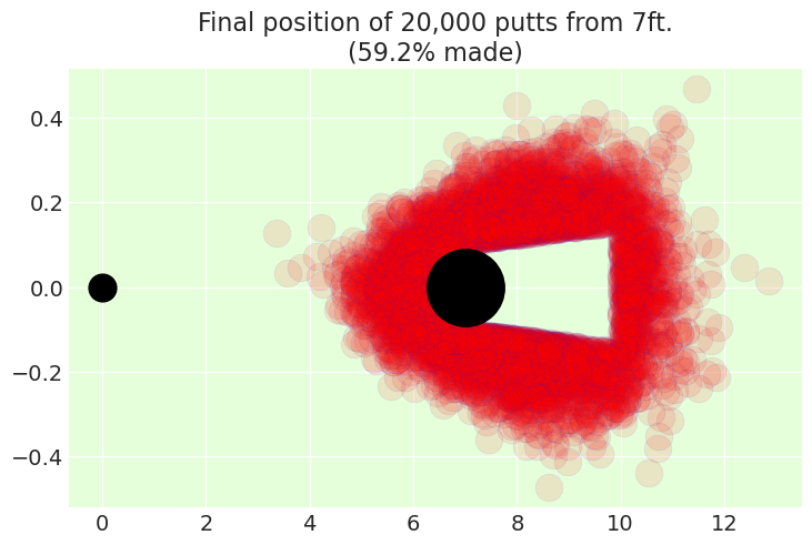
我们希望使用贝叶斯分析，因为我们关心量化参数中的不确定性。我们有一个漂亮的几何模型，它不仅为我们提供了预测，还为我们提供了参数的后验分布。我们可以使用它来推断出我们的推杆可能在哪里结束，即使没有入洞！

首先，我们可以尝试可视化职业高尔夫球手的 20,000 次推杆可能是什么样子。我们

1. 将试验次数设置为 5

2. 对于 variance_of_shot 和 variance_of_distance 的每个联合后验样本，从正态分布中抽取角度和距离 5 次。

3. 绘制该点，除非它会入洞

def simulate_from_distance(trace, distance_to_hole, trials=5):
    variance_of_shot = trace.posterior["variance_of_shot"]
    variance_of_distance = trace.posterior["variance_of_distance"]

    theta = XrContinuousRV(st.norm, 0, variance_of_shot).rvs(size=trials, dims="trials")
    distance = XrContinuousRV(
        st.norm, distance_to_hole + OVERSHOT, (distance_to_hole + OVERSHOT) * variance_of_distance
    ).rvs(size=trials, dims="trials")

    final_position = xr.concat(
        (distance * np.cos(theta), distance * np.sin(theta)), dim="axis"
    ).assign_coords(axis=["x", "y"])

    made_it = np.abs(theta) < np.arcsin((CUP_RADIUS - BALL_RADIUS) / distance_to_hole)
    made_it = (
        made_it
        * (final_position.sel(axis="x") > distance_to_hole)
        * (final_position.sel(axis="x") < distance_to_hole + DISTANCE_TOLERANCE)
    )

    dims = [dim for dim in final_position.dims if dim != "axis"]
    final_position = final_position.where(~made_it).stack(idx=dims).dropna(dim="idx")
    total_simulations = made_it.size

    _, ax = plt.subplots()

    ax.plot(0, 0, "k.", lw=1, mfc="black", ms=250 / distance_to_hole)
    ax.plot(*final_position, ".", alpha=0.1, mfc="r", ms=250 / distance_to_hole, mew=0.5)
    ax.plot(distance_to_hole, 0, "ko", lw=1, mfc="black", ms=350 / distance_to_hole)

    ax.set_facecolor("#e6ffdb")
    ax.set_title(
        f"Final position of {total_simulations:,d} putts from {distance_to_hole}ft.\n"
        f"({100 * made_it.mean().item():.1f}% made)"
    )
    return ax


simulate_from_distance(distance_angle_trace, distance_to_hole=50);

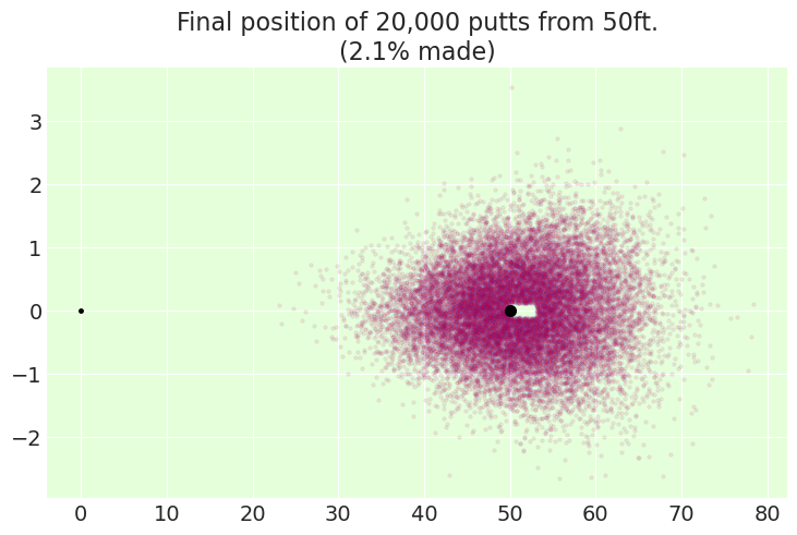
simulate_from_distance(distance_angle_trace, distance_to_hole=7);

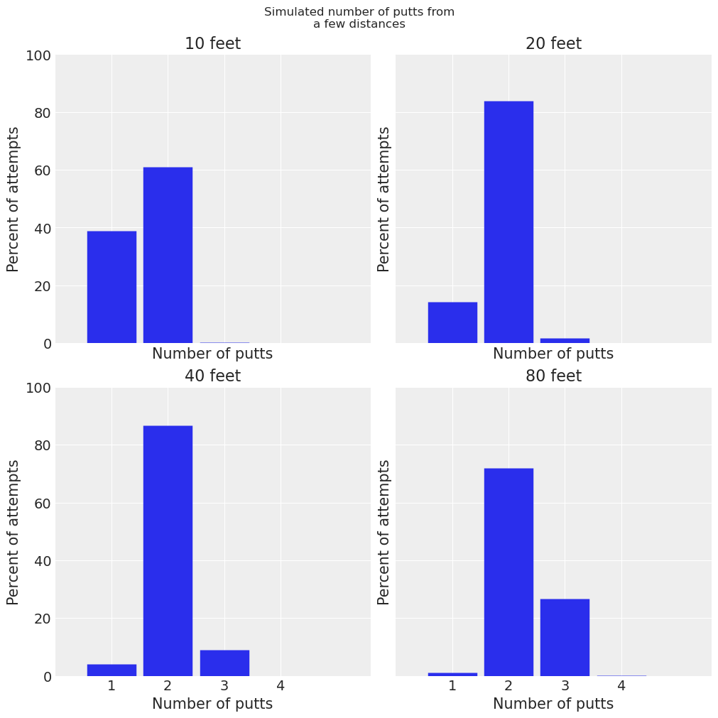
然后，我们可以使用它来计算出球员可能需要从给定距离推杆多少次。这可能会影响战略决策，例如尝试用更少的杆数到达果岭，这可能会导致第一次推杆更远，而不是更保守的方法。我们通过模拟推杆直到它们全部入洞来做到这一点。

请注意，这又是我们可以通过实验检查的东西。特别是，在互联网上进行的高度不科学的搜索发现，专业人士从 20-25 英尺处三推的次数仅占 3% 左右。我们的模型将从 22.5 英尺处 3 次或更多次推杆的机会定为 2.8%，这看起来好得令人怀疑。

def expected_num_putts(trace, distance_to_hole, trials=100_000):
    distance_to_hole = distance_to_hole * np.ones(trials)

    combined_trace = az.extract(trace)

    n_samples = combined_trace.dims["sample"]

    idxs = np.random.randint(0, n_samples, trials)
    variance_of_shot = combined_trace["variance_of_shot"].isel(sample=idxs)
    variance_of_distance = combined_trace["variance_of_distance"].isel(sample=idxs)
    n_shots = []
    while distance_to_hole.size > 0:
        theta = np.random.normal(0, variance_of_shot)
        distance = np.random.normal(
            distance_to_hole + OVERSHOT, (distance_to_hole + OVERSHOT) * variance_of_distance
        )

        final_position = np.array([distance * np.cos(theta), distance * np.sin(theta)])

        made_it = np.abs(theta) < np.arcsin(
            (CUP_RADIUS - BALL_RADIUS) / distance_to_hole.clip(min=CUP_RADIUS - BALL_RADIUS)
        )
        made_it = (
            made_it
            * (final_position[0] > distance_to_hole)
            * (final_position[0] < distance_to_hole + DISTANCE_TOLERANCE)
        )

        distance_to_hole = np.sqrt(
            (final_position[0] - distance_to_hole) ** 2 + final_position[1] ** 2
        )[~made_it].copy()
        variance_of_shot = variance_of_shot[~made_it]
        variance_of_distance = variance_of_distance[~made_it]
        n_shots.append(made_it.sum())
    return np.array(n_shots) / trials

distances = (10, 20, 40, 80)
fig, axes = plt.subplots(nrows=2, ncols=2, sharex=True, sharey=True, figsize=(10, 10))

for distance, ax in zip(distances, axes.ravel()):
    made = 100 * expected_num_putts(disp_distance_angle_trace, distance)
    x = np.arange(1, 1 + len(made), dtype=int)
    ax.vlines(np.arange(1, 1 + len(made)), 0, made, linewidths=50)
    ax.set_title(f"{distance} feet")
    ax.set_ylabel("Percent of attempts")
    ax.set_xlabel("Number of putts")
ax.set_xticks(x)
ax.set_ylim(0, 100)
ax.set_xlim(0, 5.6)
fig.suptitle("Simulated number of putts from\na few distances");

作者

• 由 Colin Carroll 根据 Stan 文档中的 [高尔夫推杆的模型构建和扩展] 案例研究改编 (pymc#3666)

• 由 Marco Gorelli 更新 (pymc-examples#39)

• 由 Oriol Abril-Pla 更新，以使用 PyMC v4 和 xarray-einstats

• 由 Benjamin T. Vincent 更新，于 2023 年 2 月使用 az.extract (pymc-examples#522)

参考文献

[1]

Donald A Berry. Statistics: a Bayesian perspective. Duxbury Press, 1996.

水印

%load_ext watermark
%watermark -n -u -v -iv -w -p aeppl,xarray_einstats

Last updated: Sun Feb 05 2023

Python implementation: CPython
Python version       : 3.10.9
IPython version      : 8.9.0

aeppl          : not installed
xarray_einstats: 0.5.1

xarray    : 2023.1.0
arviz     : 0.14.0
numpy     : 1.24.1
matplotlib: 3.6.3
pymc      : 5.0.1
scipy     : 1.10.0
pandas    : 1.5.3
pytensor  : 2.8.11

Watermark: 2.3.1

许可证声明

此示例画廊中的所有 notebook 均根据 MIT 许可证提供，该许可证允许修改和再分发以用于任何用途，前提是保留版权和许可证声明。

引用 PyMC 示例

要引用此 notebook，请使用 Zenodo 为 pymc-examples 存储库提供的 DOI。

重要提示

许多 notebook 改编自其他来源：博客、书籍... 在这种情况下，您也应该引用原始来源。

另请记住引用您的代码使用的相关库。

这是一个 bibtex 中的引用模板

@incollection{citekey,
  author    = "<notebook authors, see above>",
  title     = "<notebook title>",
  editor    = "PyMC Team",
  booktitle = "PyMC examples",
  doi       = "10.5281/zenodo.5654871"
}

渲染后可能看起来像