克罗内克结构协方差#

PyMC 包含了针对具有克罗内克结构协方差的模型的实现。这种模式化的结构使得高斯过程模型能够处理更大的数据集。在以下情况下，可以利用克罗内克结构：

输入数据的维度为两个或更多 (\(\mathbf{x} \in \mathbb{R}^{d}\,, d \ge 2\))
过程在每个维度或维度集合上的影响是可分离的
核函数可以写成维度上的乘积，而没有交叉项

\[k(\mathbf{x}, \mathbf{x'}) = \prod_{i = 1}^{d} k(\mathbf{x}_{i}, \mathbf{x'}_i) \,.\]

与上述协方差函数对应的协方差矩阵可以用克罗内克积来表示

\[ \mathbf{K} = \mathbf{K}_2 \otimes \mathbf{K}_2 \otimes \cdots \otimes \mathbf{K}_d \,. \]

这些实现支持克罗内克积的以下性质来加速计算，\((\mathbf{K}_1 \otimes \mathbf{K}_2)^{-1} = \mathbf{K}_{1}^{-1} \otimes \mathbf{K}_{2}^{-1}\)，即和的逆等于逆的和。如果 \(K_1\) 是 \(n \times n\) 矩阵，\(K_2\) 是 \(m \times m\) 矩阵，那么 \(\mathbf{K}_1 \otimes \mathbf{K}_2\) 是 \(mn \times mn\) 矩阵。对于即使是适度大小的 m 和 n，直接计算这个逆矩阵也会变得非常低效。而分别求两个矩阵的逆，一个是 \(n \times n\) 矩阵，另一个是 \(m \times m\) 矩阵，则要容易得多。

这种结构在时空数据中很常见。鉴于协方差矩阵中存在克罗内克结构，这种实现是精确的，而不是对完整高斯过程的近似。PyMC 包含两个实现，它们遵循与 gp.Marginal 和 gp.Latent 相同的模式。对于数据似然为高斯分布的克罗内克结构协方差，请使用 gp.MarginalKron。对于数据似然为非高斯分布的克罗内克结构协方差，请使用 gp.LatentKron。

我们的实现遵循 Saatchi 的论文。gp.MarginalKron 遵循使用特征分解的“算法 16”，而 gp.LatentKron 遵循“算法 14”，并使用 Cholesky 分解。

将 MarginalKron 用于二维空间问题#

以下是 gp.MarginalKron 用法的典型示例。与 gp.Marginal 类似，此模型假设底层的 GP 是未被观测到的，但 GP 和正态分布噪声的总和是被观测到的。

对于模拟数据集，我们从一个输入为二维的高斯过程中抽取一个样本，该高斯过程的协方差是克罗内克结构的。然后我们使用 gp.MarginalKron 来恢复用于模拟数据的未知高斯过程超参数 \(\theta\)。

示例#

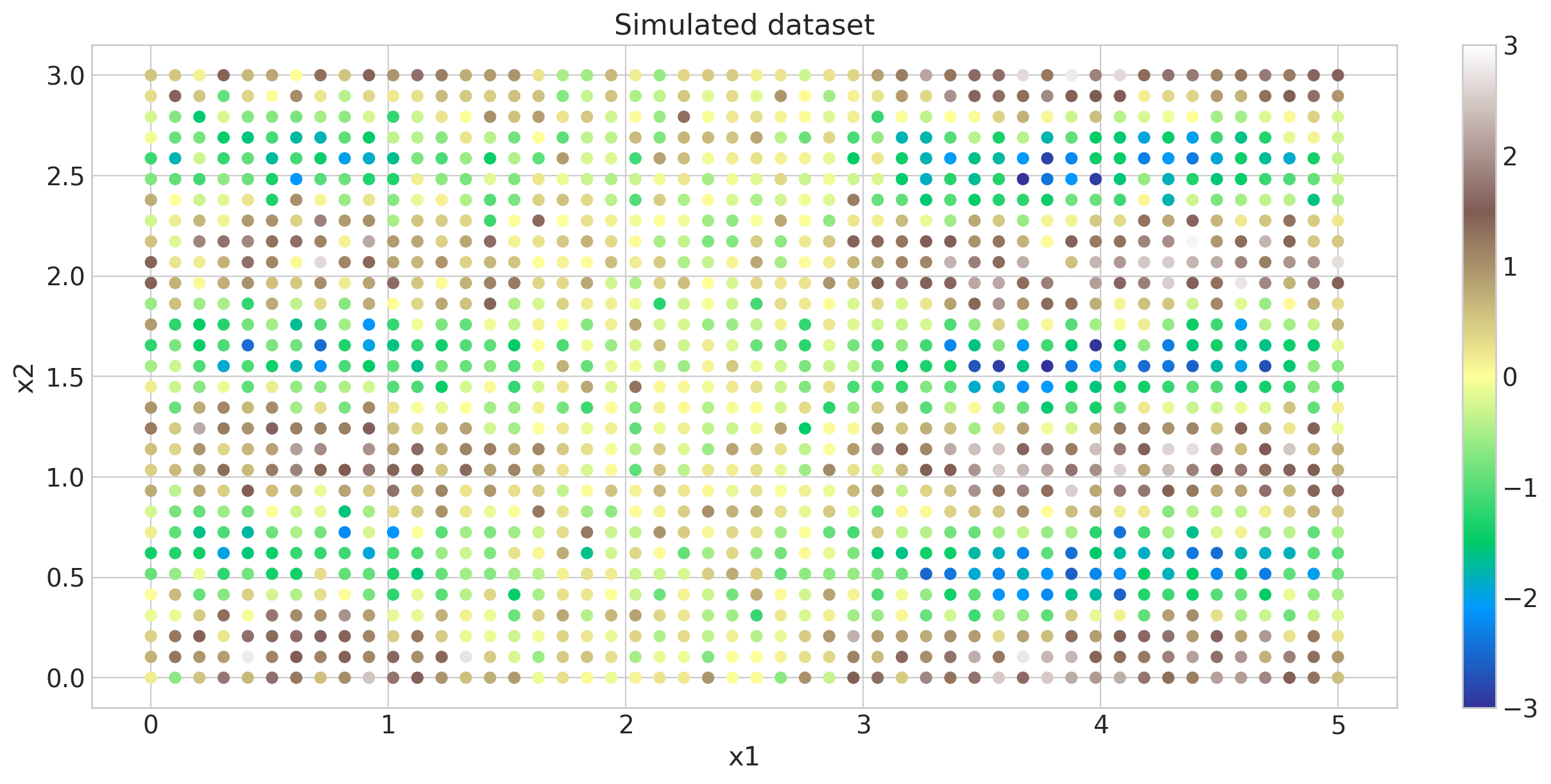
我们将模拟一个二维数据集，并将其显示为散点图，其中的点根据其大小着色。这两个维度标记为 x1 和 x2。例如，这可能是一个空间数据集。由于这些点位于二维网格上，因此协方差将具有克罗内克结构。

import arviz as az
import matplotlib as mpl
import numpy as np
import pymc as pm

az.style.use("arviz-whitegrid")
plt = mpl.pyplot
%matplotlib inline
%config InlineBackend.figure_format = 'retina'
seed = sum(map(ord, "gpkron"))
rng = np.random.default_rng(seed)

# One dimensional column vectors of inputs
n1, n2 = (50, 30)
x1 = np.linspace(0, 5, n1)
x2 = np.linspace(0, 3, n2)

# make cartesian grid out of each dimension x1 and x2
X = pm.math.cartesian(x1[:, None], x2[:, None])

l1_true = 0.8
l2_true = 1.0
eta_true = 1.0

# Although we could, we don't exploit kronecker structure to draw the sample
cov = (
    eta_true**2
    * pm.gp.cov.Matern52(2, l1_true, active_dims=[0])
    * pm.gp.cov.Cosine(2, ls=l2_true, active_dims=[1])
)

K = cov(X).eval()
f_true = rng.multivariate_normal(np.zeros(X.shape[0]), K, 1).flatten()

sigma_true = 0.5
y = f_true + sigma_true * rng.standard_normal(X.shape[0])

沿 x2 维度的长度尺度比沿 x1 方向的长度尺度更长 (l1_true < l2_true)。

fig = plt.figure(figsize=(12, 6))
cmap = "terrain"
norm = mpl.colors.Normalize(vmin=-3, vmax=3)
plt.scatter(X[:, 0], X[:, 1], s=35, c=y, marker="o", norm=norm, cmap=cmap)
plt.colorbar()
plt.xlabel("x1"), plt.ylabel("x2")
plt.title("Simulated dataset");

../_images/9435fadf9974988d30272358b4362f3668eaf3d471533a2c5a524717d68ce709.png

此数据集中有 1500 个数据点。如果不使用克罗内克分解，找到 MAP 估计会慢得多。

由于这两个协方差是乘积，我们只需要一个尺度参数 eta 来建模乘积协方差函数。

# this implementation takes a list of inputs for each dimension as input
Xs = [x1[:, None], x2[:, None]]

with pm.Model() as model:
    # Set priors on the hyperparameters of the covariance
    ls1 = pm.Gamma("ls1", alpha=2, beta=2)
    ls2 = pm.Gamma("ls2", alpha=2, beta=2)
    eta = pm.HalfNormal("eta", sigma=2)

    # Specify the covariance functions for each Xi
    # Since the covariance is a product, only scale one of them by eta.
    # Scaling both overparameterizes the covariance function.
    cov_x1 = pm.gp.cov.Matern52(1, ls=ls1)  # cov_x1 must accept X1 without error
    cov_x2 = eta**2 * pm.gp.cov.Cosine(1, ls=ls2)  # cov_x2 must accept X2 without error

    # Specify the GP.  The default mean function is `Zero`.
    gp = pm.gp.MarginalKron(cov_funcs=[cov_x1, cov_x2])

    # Set the prior on the variance for the Gaussian noise
    sigma = pm.HalfNormal("sigma", sigma=2)

    # Place a GP prior over the function f.
    y_ = gp.marginal_likelihood("y", Xs=Xs, y=y, sigma=sigma)

with model:
    mp = pm.find_MAP(method="BFGS")

mp

{'ls1_log__': array(0.13716063),
 'ls2_log__': array(-0.0004206),
 'eta_log__': array(0.34822276),
 'sigma_log__': array(-0.65839497),
 'ls1': array(1.14701237),
 'ls2': array(0.99957949),
 'eta': array(1.41654776),
 'sigma': array(0.51768156)}

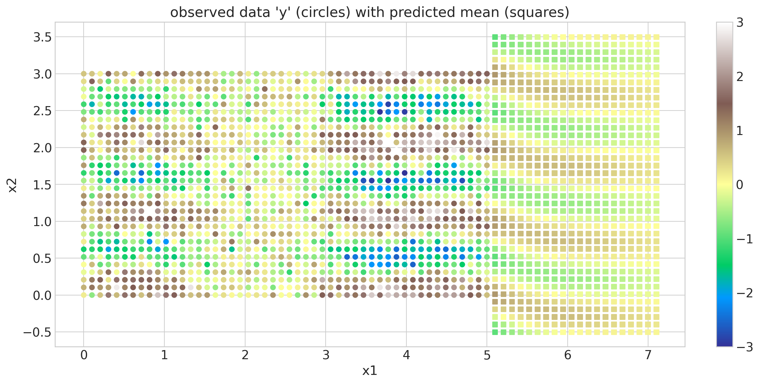
接下来，我们使用 map point mp 在原始网格外部的区域进行外推。我们也可以进行内插。对于期望预测的新输入，没有网格限制。重要的是要注意，在当前的实现下，在这些点中具有网格结构不会产生任何效率提升。带有外推的图显示在下面。原始数据像以前一样用圆圈标记，但外推的后验均值用正方形标记。

x1new = np.linspace(5.1, 7.1, 20)
x2new = np.linspace(-0.5, 3.5, 40)
Xnew = pm.math.cartesian(x1new[:, None], x2new[:, None])

with model:
    mu, var = gp.predict(Xnew, point=mp, diag=True)

fig = plt.figure(figsize=(12, 6))
cmap = "terrain"
norm = mpl.colors.Normalize(vmin=-3, vmax=3)
m = plt.scatter(X[:, 0], X[:, 1], s=30, c=y, marker="o", norm=norm, cmap=cmap)
plt.colorbar(m)
plt.scatter(Xnew[:, 0], Xnew[:, 1], s=30, c=mu, marker="s", norm=norm, cmap=cmap)
plt.ylabel("x2"), plt.xlabel("x1")
plt.title("observed data 'y' (circles) with predicted mean (squares)");

../_images/605deeb9a5cd05d41f170b5c49ddad6f2a9ac06f9da7d90ebe8e9358f179153d.png

`LatentKron`#

与 gp.Latent 实现类似，gp.LatentKron 实现指定了一个克罗内克结构化的 GP，而与上下文无关。它可以与任何似然函数一起使用，也可以用于建模方差或某些其他未观测到的过程。其语法与 gp.Latent 完全相同。

模型#

为了与 MarginalLikelihood 进行比较，我们使用与之前相同的示例，其中噪声是正态的，但 GP 本身没有被边缘化。相反，它是使用 NUTS 直接采样的。非常重要的是要注意，gp.LatentKron 不需要像 gp.MarginalKron 那样的高斯似然；相反，任何似然都是允许的。

然而，在这里，我们需要为我们的先验提供更多信息，至少是 GP 超参数的先验。这是使用 GP 时的一般规则：尽可能使用信息量丰富的先验，因为对长度尺度和幅度进行采样是一项具有挑战性的任务，因此您希望尽可能简化采样器的工作。

谢天谢地，我们这里有很多关于我们的幅度和长度尺度的信息——我们是创建它们的人 ;) 所以我们可以固定它们，但我们将展示如何在您自己的模型中编码先验知识，例如，使用截断正态分布

with pm.Model() as model:
    # Set priors on the hyperparameters of the covariance
    ls1 = pm.TruncatedNormal("ls1", lower=0.5, upper=1.5, mu=1, sigma=0.5)
    ls2 = pm.TruncatedNormal("ls2", lower=0.5, upper=1.5, mu=1, sigma=0.5)
    eta = pm.HalfNormal("eta", sigma=0.5)

    # Specify the covariance functions for each Xi
    cov_x1 = pm.gp.cov.Matern52(1, ls=ls1)
    cov_x2 = eta**2 * pm.gp.cov.Cosine(1, ls=ls2)

    # Specify the GP. The default mean function is `Zero`
    gp = pm.gp.LatentKron(cov_funcs=[cov_x1, cov_x2])

    # Place a GP prior over the function f
    f = gp.prior("f", Xs=Xs)

    # Set the prior on the variance for the Gaussian noise
    sigma = pm.HalfNormal("sigma", sigma=0.5)

    y_ = pm.Normal("y_", mu=f, sigma=sigma, observed=y)

pm.model_to_graphviz(model)

../_images/f47ff99a7109188e15e5f39c15c8da84c90d147a307587f333bed35406ebe1f2.svg

with model:
    idata = pm.sample(nuts_sampler="numpyro", target_accept=0.9, tune=1500, draws=1500)

idata.sample_stats.diverging.sum().data

array(0)

后验收敛#

未知长度尺度参数、协方差缩放 eta 和白噪声 sigma 的后验分布如下所示。垂直线是用于生成原始数据集的真实值

var_names = ["ls1", "ls2", "eta", "sigma"]

az.plot_posterior(
    idata,
    var_names=var_names,
    ref_val=[l1_true, l2_true, eta_true, sigma_true],
    grid=(2, 2),
    figsize=(12, 6),
);

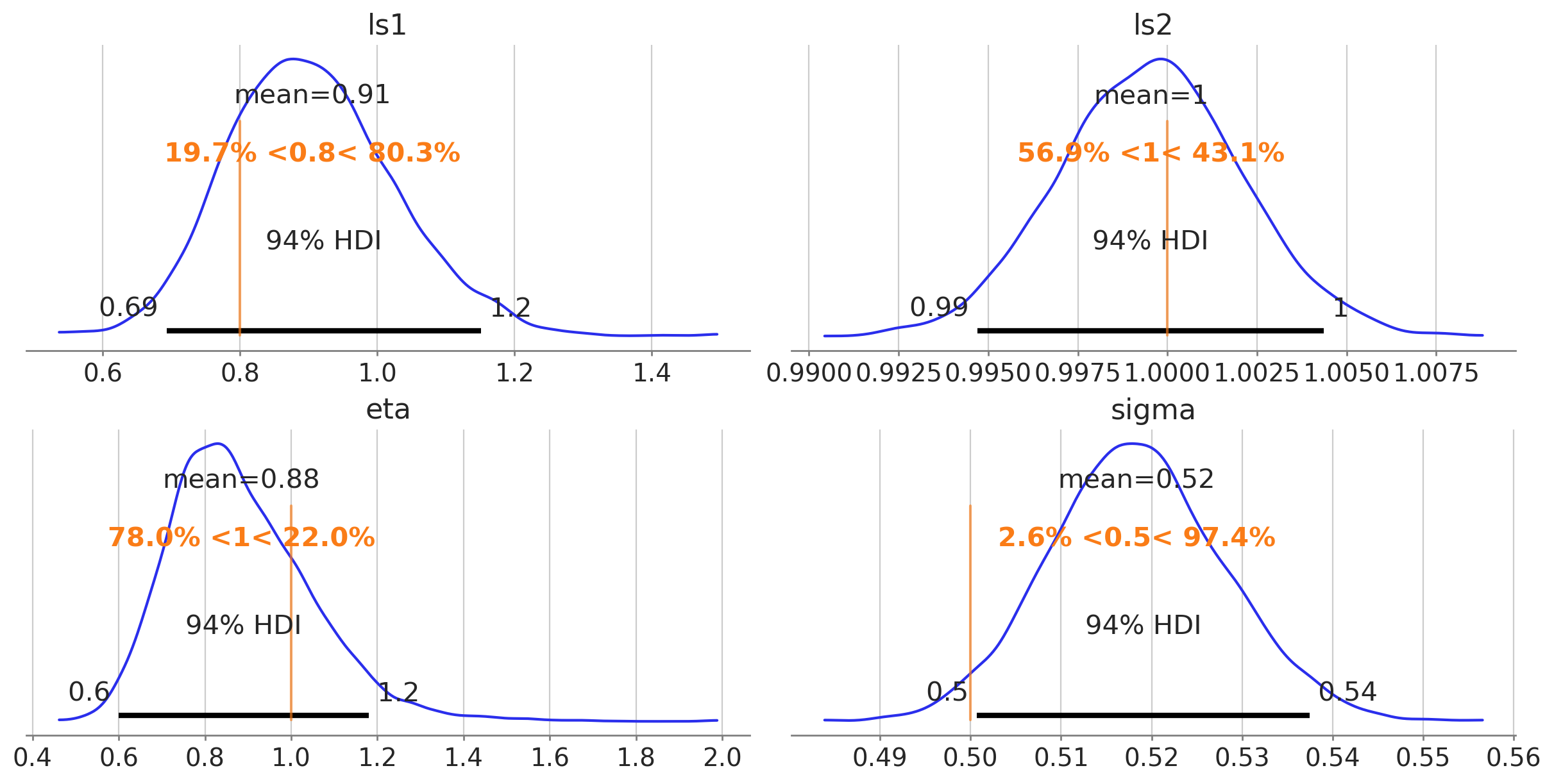
../_images/e10e6d9e71e02bbde1cd55745fe67d0122cf98041a35ef454e6661ff82441e54.png

我们可以看到在这些情况下采样可能有多么具有挑战性。在这里，一切进展顺利，因为我们对先验的选择非常谨慎——尤其是在这种模拟情况下，参数没有实际的解释。

轨迹图看起来怎么样？

az.plot_trace(idata, var_names=var_names);

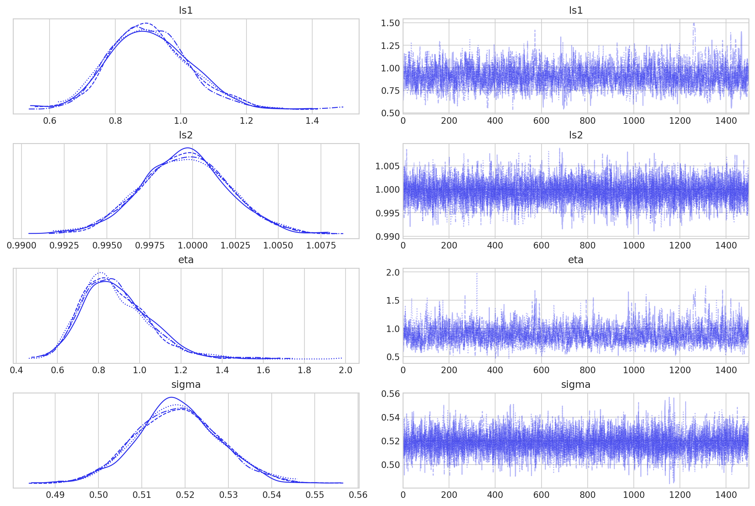
../_images/6873efdf8ee6f083ce325c5922ff88f826bcfc3f737bbcd0ca4713537205c6ee.png

一切都很好，那么让我们继续进行样本外预测！

样本外预测#

x1new = np.linspace(5.1, 7.1, 20)[:, None]
x2new = np.linspace(-0.5, 3.5, 40)[:, None]
Xnew = pm.math.cartesian(x1new, x2new)
x1new.shape, x2new.shape, Xnew.shape

((20, 1), (40, 1), (800, 2))

with model:
    fnew = gp.conditional("fnew", Xnew, jitter=1e-6)

with model:
    ppc = pm.sample_posterior_predictive(idata, var_names=["fnew"], compile_kwargs={"mode": "JAX"})

/Users/alex_andorra/mambaforge/envs/pymc-examples/lib/python3.12/site-packages/pytensor/link/jax/linker.py:28: UserWarning: The RandomType SharedVariables [RandomGeneratorSharedVariable(<Generator(PCG64) at 0x17B535D20>)] will not be used in the compiled JAX graph. Instead a copy will be used.
  warnings.warn(
Sampling: [fnew]

2024-05-27 15:30:56.157723: E external/xla/xla/service/slow_operation_alarm.cc:65] Constant folding an instruction is taking > 1s:

  %reduce.3 = f64[1500,800]{1,0} reduce(f64[1,1500,800]{2,1,0} %broadcast.59, f64[] %constant.76), dimensions={0}, to_apply=%region_2.198, metadata={op_name="jit(jax_funcified_fgraph)/jit(main)/reduce_sum[axes=(0,)]" source_file="/var/folders/m_/brf3tky55f3gf6dy8w7c6s0w0000gn/T/tmpnlsq8yzu" source_line=77}

This isn't necessarily a bug; constant-folding is inherently a trade-off between compilation time and speed at runtime. XLA has some guards that attempt to keep constant folding from taking too long, but fundamentally you'll always be able to come up with an input program that takes a long time.

If you'd like to file a bug, run with envvar XLA_FLAGS=--xla_dump_to=/tmp/foo and attach the results.
2024-05-27 15:30:56.305845: E external/xla/xla/service/slow_operation_alarm.cc:133] The operation took 1.153176s
Constant folding an instruction is taking > 1s:

  %reduce.3 = f64[1500,800]{1,0} reduce(f64[1,1500,800]{2,1,0} %broadcast.59, f64[] %constant.76), dimensions={0}, to_apply=%region_2.198, metadata={op_name="jit(jax_funcified_fgraph)/jit(main)/reduce_sum[axes=(0,)]" source_file="/var/folders/m_/brf3tky55f3gf6dy8w7c6s0w0000gn/T/tmpnlsq8yzu" source_line=77}

This isn't necessarily a bug; constant-folding is inherently a trade-off between compilation time and speed at runtime. XLA has some guards that attempt to keep constant folding from taking too long, but fundamentally you'll always be able to come up with an input program that takes a long time.

If you'd like to file a bug, run with envvar XLA_FLAGS=--xla_dump_to=/tmp/foo and attach the results.

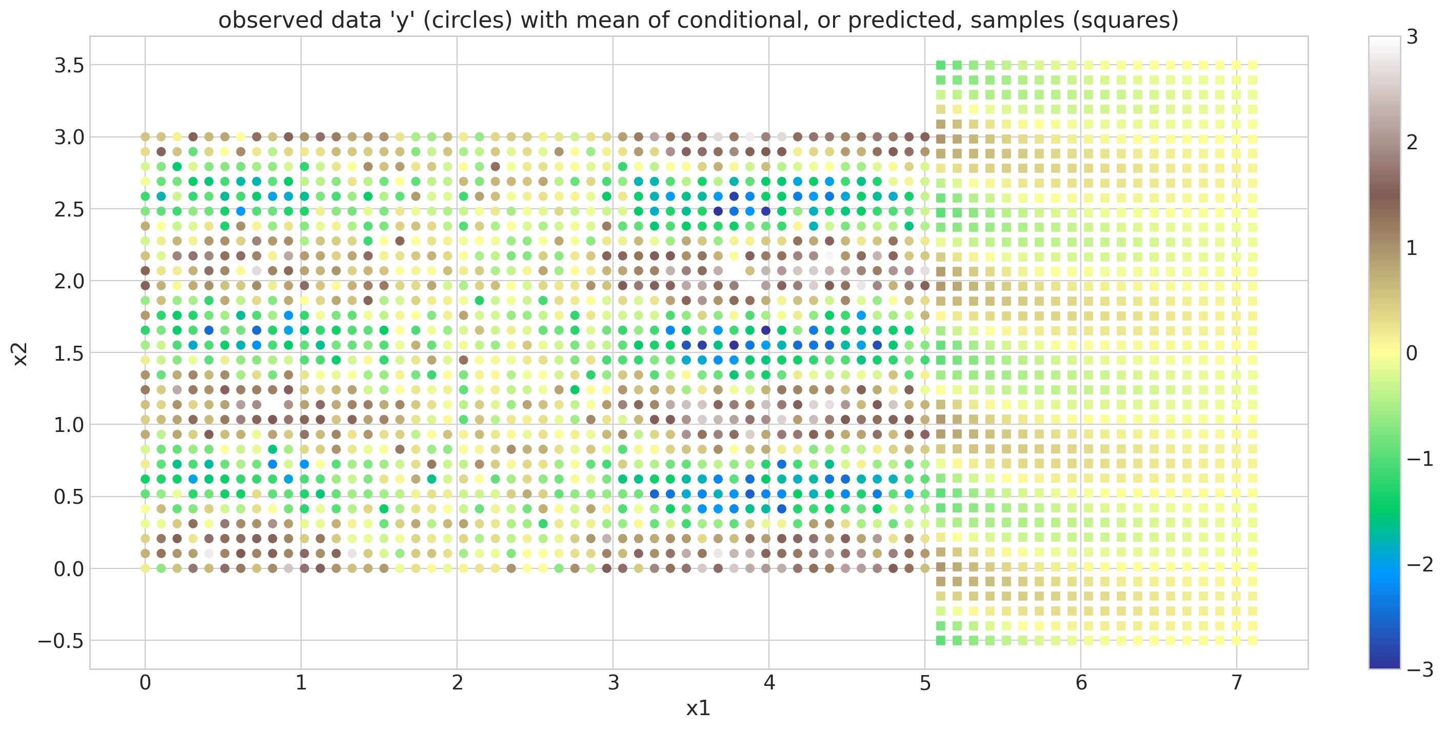
下面我们显示了原始数据集，用彩色圆圈表示，以及条件样本的均值，用彩色正方形表示。结果与 gp.MarginalKron 实现给出的结果非常接近。

fig = plt.figure(figsize=(14, 7))
m = plt.scatter(X[:, 0], X[:, 1], s=30, c=y, marker="o", norm=norm, cmap=cmap)
plt.colorbar(m)
plt.scatter(
    Xnew[:, 0],
    Xnew[:, 1],
    s=30,
    c=np.mean(ppc.posterior_predictive["fnew"].sel(chain=0), axis=0),
    marker="s",
    norm=norm,
    cmap=cmap,
)
plt.ylabel("x2"), plt.xlabel("x1")
plt.title("observed data 'y' (circles) with mean of conditional, or predicted, samples (squares)");

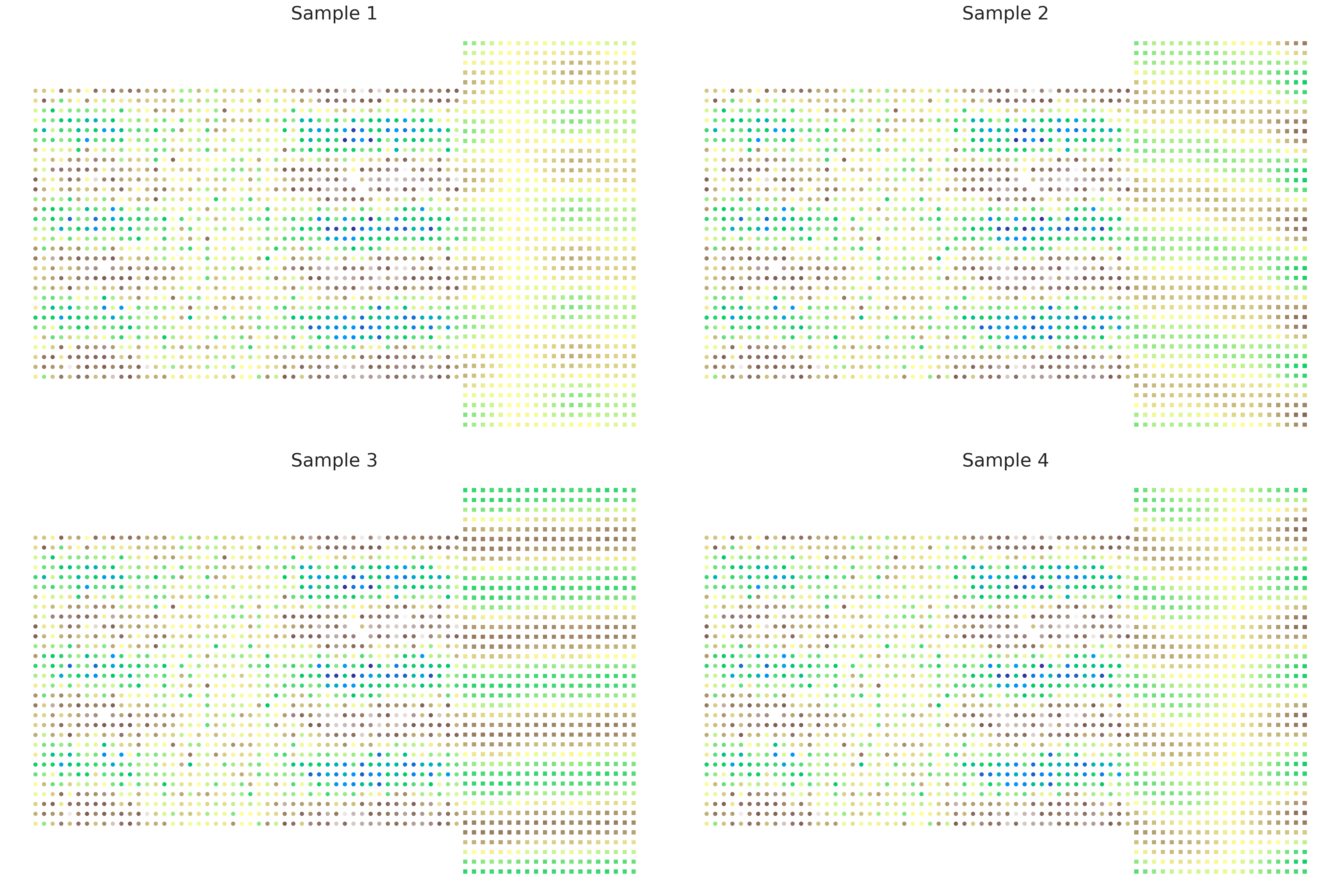
../_images/a88e5b21588fbd088a298c58b7709656197390fa9e8f6ea96c3d07de5c3dc2e6.png

接下来，我们绘制了原始数据集，用圆圈标记表示，以及来自 fnew 条件分布的四个样本，用正方形标记表示。正如我们所看到的，预测分布中的变异水平导致 fnew 值中出现明显不同的模式。然而，这些样本显示了正确的相关结构——我们看到 y 轴上明显的正弦模式和 x 轴上的近端相关结构。观测数据中显示的模式无缝地融入到条件分布中。

fig, axs = plt.subplots(2, 2, figsize=(24, 16))
axs = axs.ravel()

for i, ax in enumerate(axs):
    ax.axis("off")
    ax.scatter(X[:, 0], X[:, 1], s=20, c=y, marker="o", norm=norm, cmap=cmap)
    ax.scatter(
        Xnew[:, 0],
        Xnew[:, 1],
        s=20,
        c=ppc.posterior_predictive["fnew"].sel(chain=0)[i],
        marker="s",
        norm=norm,
        cmap=cmap,
    )
    ax.set_title(f"Sample {i+1}", fontsize=24)

../_images/5f150e7d9135fc50a051d892d947ef7aeb100703770646313d588f5f2f2a0105.png

作者#

由 Bill Engels 编写，2018
由 Raul-ing Average 更新，2021 年 3 月
由 Christopher Krapu 更新，2021 年 7 月
由 Danh Phan 更新至 PyMC 4.x，2022 年 11 月
由 Alex Andorra 更新，添加了一些新图表和先验，2024 年 4 月

水印#

%load_ext watermark
%watermark -n -u -v -iv -w -p pytensor,xarray

Last updated: Mon May 27 2024

Python implementation: CPython
Python version       : 3.12.2
IPython version      : 8.22.2

pytensor: 2.20.0
xarray  : 2024.3.0

numpy     : 1.26.4
pymc      : 5.15.0+14.gfd11cf012
arviz     : 0.17.1
matplotlib: 3.8.3

Watermark: 2.4.3

许可证声明#

本示例库中的所有 Notebook 均根据 MIT 许可证提供，该许可证允许修改和再分发以用于任何用途，前提是保留版权和许可证声明。

引用 PyMC 示例#

要引用此 Notebook，请使用 Zenodo 为 pymc-examples 存储库提供的 DOI。

重要提示

许多 Notebook 改编自其他来源：博客、书籍…… 在这种情况下，您也应该引用原始来源。

还请记住引用您的代码使用的相关库。

这是一个 bibtex 格式的引用模板

@incollection{citekey,
  author    = "<notebook authors, see above>",
  title     = "<notebook title>",
  editor    = "PyMC Team",
  booktitle = "PyMC examples",
  doi       = "10.5281/zenodo.5654871"
}

渲染后可能看起来像这样

分类

标签

克罗内克结构协方差#

将 MarginalKron 用于二维空间问题#

示例#

`LatentKron`#

模型#

后验收敛#

样本外预测#

作者#

水印#

许可证声明#

引用 PyMC 示例#

分类

标签

克罗内克结构协方差#

将 MarginalKron 用于二维空间问题#

示例#

LatentKron#

模型#

后验收敛#

样本外预测#

作者#

水印#

许可证声明#

引用 PyMC 示例#

`LatentKron`#