


高斯过程:隐变量实现#
gp.Latent 类是高斯过程的直接实现,无需近似。给定均值和协方差函数,我们可以对函数 \(f(x)\) 设置先验,
它被称为“隐变量”,因为 GP 本身作为隐变量包含在模型中,它不像 gp.Marginal 那样被边缘化处理。与 gp.Latent 不同,您不会在 gp.Marginal 的迹中找到来自 GP 后验的样本。这是 GP 最直接的实现,因为它不假设特定的似然函数或数据或协方差矩阵中的结构。
.prior 方法#
prior 方法将多元正态先验分布添加到 PyMC 模型中,分布对象是 GP 函数值向量 \(\mathbf{f}\),
其中向量 \(\mathbf{m}_x\) 和矩阵 \(\mathbf{K}_{xx}\) 是在输入 \(x\) 上评估的均值向量和协方差矩阵。默认情况下,PyMC 通过使用协方差矩阵的 Cholesky 因子旋转 f 上的先验来进行重参数化。这通过减少变换后的随机变量 v 的后验协方差来改进采样。重参数化模型为:
有关此重参数化的更多信息,请参阅关于从多元分布中抽取值的部分。
.conditional 方法#
conditional 方法实现了函数值的预测分布,这些函数值不是原始数据集的一部分。此分布为:
使用我们上面定义的相同 gp 对象,我们可以通过以下方式构造具有此分布的随机变量:
# vector of new X points we want to predict the function at
X_star = np.linspace(0, 2, 100)[:, None]

with latent_gp_model:
    f_star = gp.conditional("f_star", X_star)
示例 1:具有 Student-T 分布噪声的回归#
以下示例展示了如何使用 gp.Latent 类指定具有 GP 先验的简单模型。我们使用 GP 生成数据,以便我们可以验证我们执行的推断是否正确。请注意,似然不是正态分布,而是 IID Student-T 分布。对于似然为高斯分布时更有效的实现,请使用 gp.Marginal。
注意
此笔记本使用了非 PyMC 依赖项的库,因此需要专门安装才能运行此笔记本。打开下面的下拉菜单以获取更多指导。
额外依赖项安装说明
为了运行此笔记本(在本地或 Binder 上),您不仅需要安装可用的 PyMC 以及所有可选依赖项,还需要安装一些额外的依赖项。有关安装 PyMC 本身的建议,请参阅 安装
您可以使用首选的软件包管理器安装这些依赖项,我们在下面提供了 pip 和 conda 命令的示例。
$ pip install jax numpyro
请注意,如果您想(或需要)从笔记本内部而不是命令行安装软件包,则可以通过运行 pip 命令的变体来安装软件包
import sys
!{sys.executable} -m pip install jax numpyro
您不应运行 !pip install,因为它可能会将软件包安装在不同的环境中,即使已安装,也无法从 Jupyter 笔记本中使用。
另一种选择是使用 conda 代替
$ conda install jax numpyro
当使用 conda 安装科学 Python 软件包时,我们建议使用 conda-forge
import arviz as az
import matplotlib.pyplot as plt
import numpy as np
import pymc as pm
%config InlineBackend.figure_format = 'retina'

RANDOM_SEED = 8998
rng = np.random.default_rng(RANDOM_SEED)

az.style.use("arviz-darkgrid")
n = 50  # The number of data points
X = np.linspace(0, 10, n)[:, None]  # The inputs to the GP must be arranged as a column vector

# Define the true covariance function and its parameters
ell_true = 1.0
eta_true = 4.0
cov_func = eta_true**2 * pm.gp.cov.ExpQuad(1, ell_true)

# A mean function that is zero everywhere
mean_func = pm.gp.mean.Zero()

# The latent function values are one sample from a multivariate normal
f_true = pm.draw(pm.MvNormal.dist(mu=mean_func(X), cov=cov_func(X)), 1, random_seed=rng)

# The observed data is the latent function plus a small amount of T distributed noise
# The standard deviation of the noise is `sigma`, and the degrees of freedom is `nu`
sigma_true = 1.0
nu_true = 5.0
y = f_true + sigma_true * rng.standard_t(df=nu_true, size=n)

## Plot the data and the unobserved latent function
fig = plt.figure(figsize=(10, 4))
ax = fig.gca()
ax.plot(X, f_true, "dodgerblue", lw=3, label="True generating function 'f'")
ax.plot(X, y, "ok", ms=3, label="Observed data")
ax.set_xlabel("X")
ax.set_ylabel("y")
plt.legend(frameon=True);
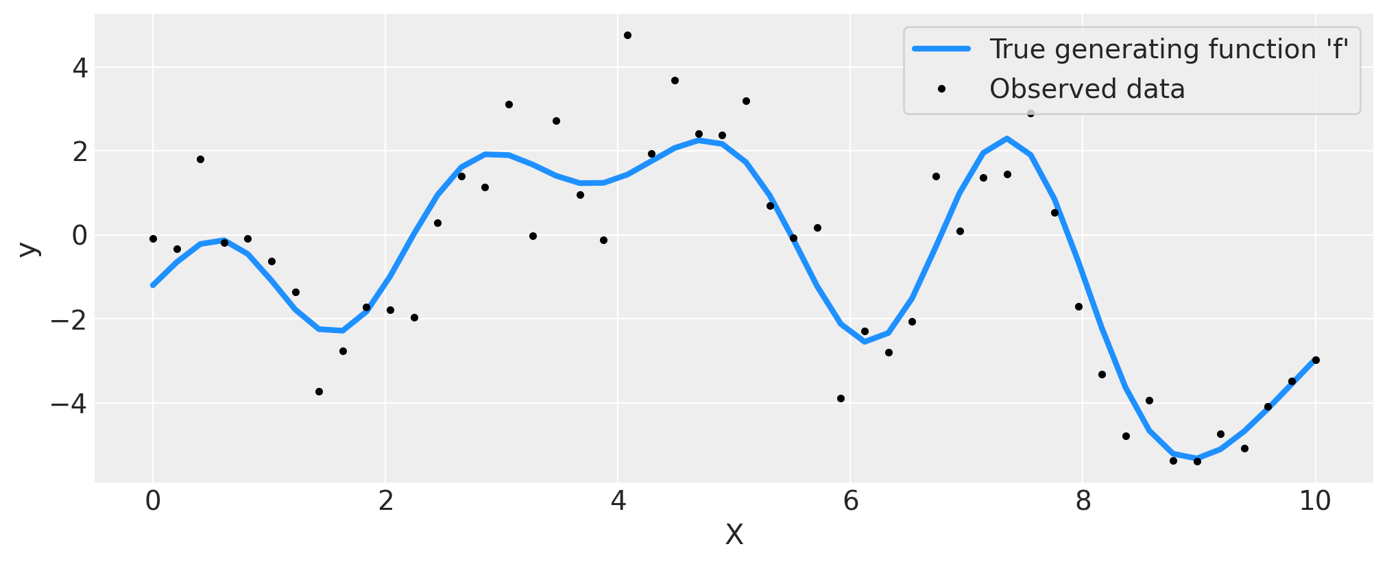
上面的数据显示了未知函数 \(f(x)\) 的观测值,用黑点标记,这些观测值已被噪声破坏。真实函数为蓝色。
在 PyMC 中编写模型代码#
这是 PyMC 中的模型。我们对长度尺度参数使用信息 pm.Gamma(alpha=2, beta=1) 先验,对协方差函数尺度和噪声尺度使用弱信息 pm.HalfNormal(sigma=5) 先验。为噪声的自由度参数分配 pm.Gamma(2, 0.5) 先验。最后,在未知函数上放置 GP 先验。有关在高斯过程模型中选择先验的更多信息,请查看 Stan 团队的一些建议。
with pm.Model() as model:
    ell = pm.Gamma("ell", alpha=2, beta=1)
    eta = pm.HalfNormal("eta", sigma=5)

    cov = eta**2 * pm.gp.cov.ExpQuad(1, ell)
    gp = pm.gp.Latent(cov_func=cov)

    f = gp.prior("f", X=X)

    sigma = pm.HalfNormal("sigma", sigma=2.0)
    nu = 1 + pm.Gamma(
        "nu", alpha=2, beta=0.1
    )  # add one because student t is undefined for degrees of freedom less than one
    y_ = pm.StudentT("y", mu=f, lam=1.0 / sigma, nu=nu, observed=y)

    idata = pm.sample(nuts_sampler="numpyro")
# check Rhat, values above 1 may indicate convergence issues
n_nonconverged = int(
    np.sum(az.rhat(idata)[["eta", "ell", "sigma", "f_rotated_"]].to_array() > 1.03).values
)
if n_nonconverged == 0:
    print("No Rhat values above 1.03, \N{check mark}")
else:
    print(f"The MCMC chains for {n_nonconverged} RVs appear not to have converged.")
No Rhat values above 1.03, ✓
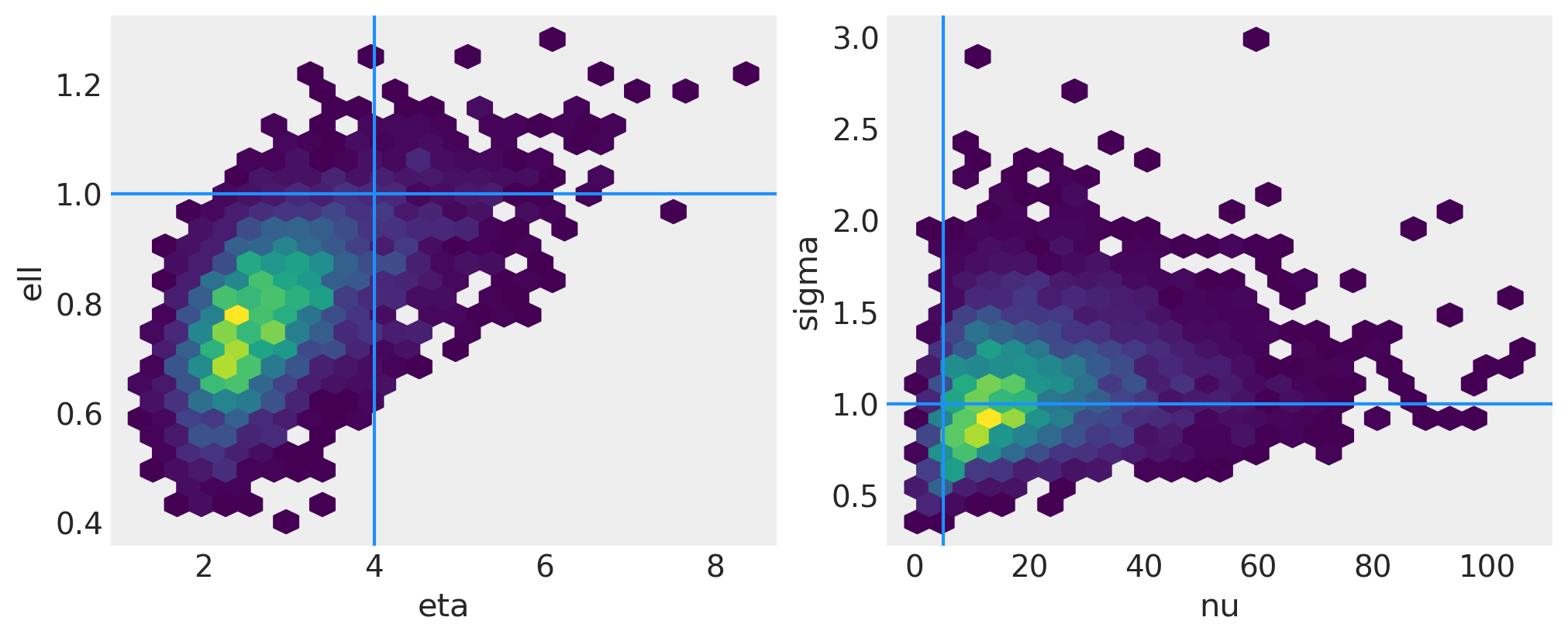
结果#
左侧面板中绘制了两个协方差函数超参数的联合后验。右侧面板是噪声的标准差和似然的自由度参数的联合后验。浅蓝色线条显示了用于从 GP 中抽取函数的真实值。
fig, axs = plt.subplots(1, 2, figsize=(10, 4))
axs = axs.flatten()

# plot eta vs ell
az.plot_pair(
    idata,
    var_names=["eta", "ell"],
    kind=["hexbin"],
    ax=axs[0],
    gridsize=25,
    divergences=True,
)
axs[0].axvline(x=eta_true, color="dodgerblue")
axs[0].axhline(y=ell_true, color="dodgerblue")

# plot nu vs sigma
az.plot_pair(
    idata,
    var_names=["nu", "sigma"],
    kind=["hexbin"],
    ax=axs[1],
    gridsize=25,
    divergences=True,
)

axs[1].axvline(x=nu_true, color="dodgerblue")
axs[1].axhline(y=sigma_true, color="dodgerblue");
f_post = az.extract(idata, var_names="f").transpose("sample", ...)
f_post
<xarray.DataArray 'f' (sample: 4000, f_dim_0: 50)> Size: 2MB
array([[-0.02178219,  0.48692574,  0.72459977, ..., -3.95601759,
        -2.98300033, -1.73010505],
       [-0.09583607,  0.51662223,  0.77188372, ..., -3.83529288,
        -3.59571791, -3.08346489],
       [ 0.28659004,  0.22130982,  0.47902239, ..., -3.7474786 ,
        -3.42978883, -3.63249247],
       ...,
       [-0.34645708,  0.32101281,  0.54055127, ..., -5.29751615,
        -4.60317113, -3.6833632 ],
       [-0.43322884,  0.25015173,  0.77657642, ..., -3.90482847,
        -3.7119477 , -3.38187578],
       [-1.0782359 , -0.83568734, -0.65140178, ..., -4.15961319,
        -3.89080578, -3.5752233 ]])
Coordinates:
  * f_dim_0  (f_dim_0) int64 400B 0 1 2 3 4 5 6 7 8 ... 42 43 44 45 46 47 48 49
  * sample   (sample) object 32kB MultiIndex
  * chain    (sample) int64 32kB 0 0 0 0 0 0 0 0 0 0 0 ... 3 3 3 3 3 3 3 3 3 3 3
* draw (sample) int64 32kB 0 1 2 3 4 5 6 7 ... 993 994 995 996 997 998 999以下是 GP 的后验,
# plot the results
fig = plt.figure(figsize=(10, 4))
ax = fig.gca()

# plot the samples from the gp posterior with samples and shading
from pymc.gp.util import plot_gp_dist

f_post = az.extract(idata, var_names="f").transpose("sample", ...)
plot_gp_dist(ax, f_post, X)

# plot the data and the true latent function
ax.plot(X, f_true, "dodgerblue", lw=3, label="True generating function 'f'")
ax.plot(X, y, "ok", ms=3, label="Observed data")

# axis labels and title
plt.xlabel("X")
plt.ylabel("True f(x)")
plt.title("Posterior distribution over $f(x)$ at the observed values")
plt.legend();
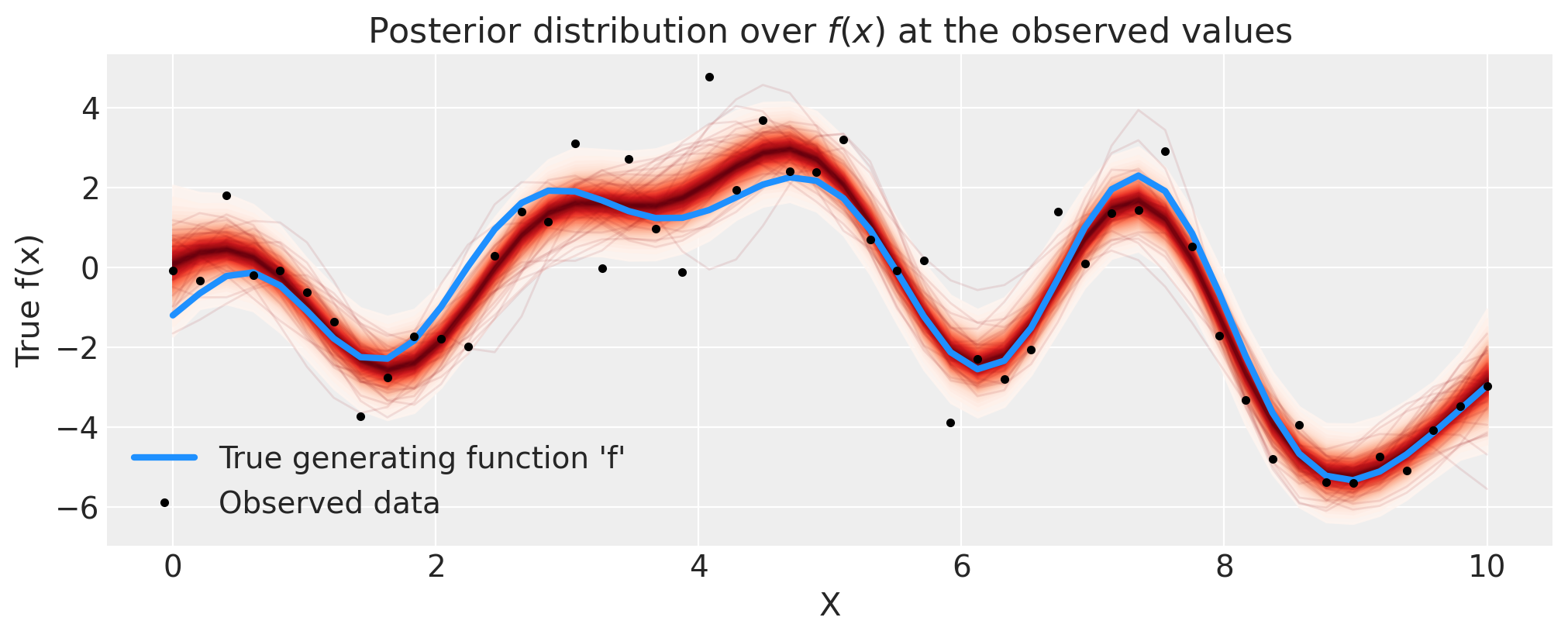
正如您可以通过红色阴影看到的那样,GP 先验在函数上的后验在表示拟合以及由加性噪声引起的不确定性方面做得非常出色。由于 Student-T 噪声模型中的异常值,结果也不会过度拟合。
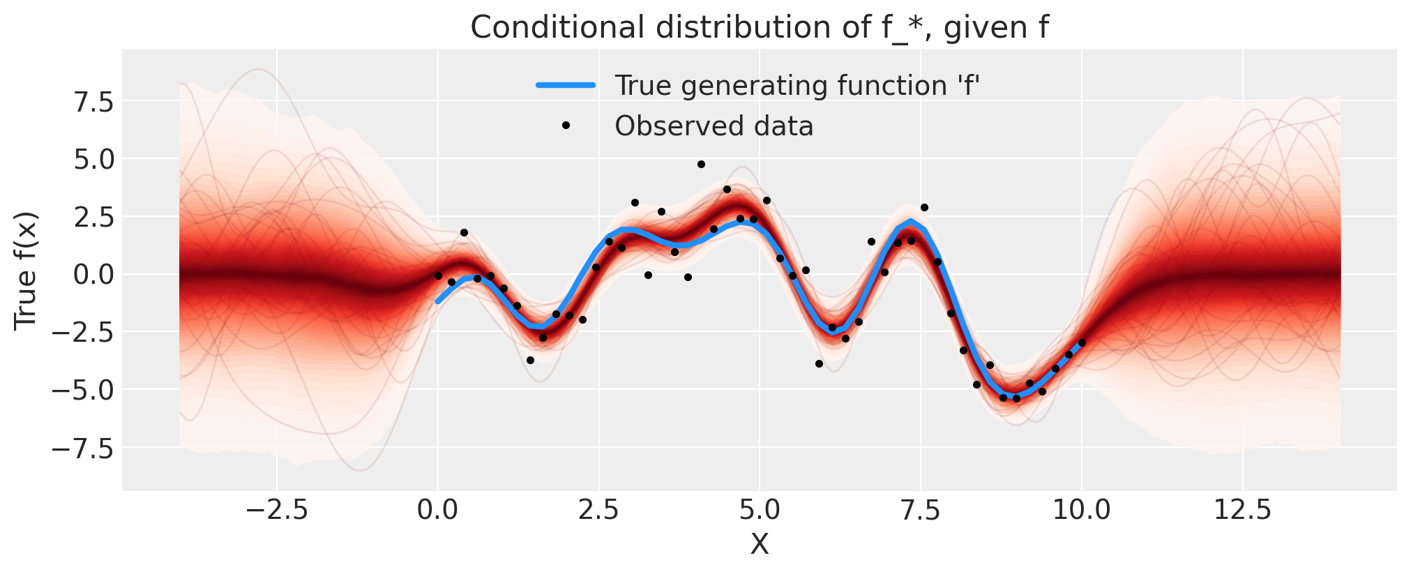
使用 .conditional 进行预测#
接下来,我们通过添加条件分布来扩展模型,以便我们可以预测新的 \(x\) 位置。让我们看看外推到更高的 \(x\) 的效果如何。为此,我们使用 GP 的 conditional 分布扩展我们的 model。然后,我们可以使用 trace 和 sample_posterior_predictive 函数从中采样。
这类似于 Stan 如何使用其 generated quantities {...} 块。我们本可以在进行 NUTS 采样之前在模型中包含 gp.conditional,但将这些步骤分开更有效率。
n_new = 200
X_new = np.linspace(-4, 14, n_new)[:, None]

with model:
    # add the GP conditional to the model, given the new X values
    f_pred = gp.conditional("f_pred", X_new, jitter=1e-4)

    # Sample from the GP conditional distribution
    idata.extend(pm.sample_posterior_predictive(idata, var_names=["f_pred"]))
Sampling: [f_pred]
fig = plt.figure(figsize=(10, 4))
ax = fig.gca()

f_pred = az.extract(idata.posterior_predictive, var_names="f_pred").transpose("sample", ...)
plot_gp_dist(ax, f_pred, X_new)

ax.plot(X, f_true, "dodgerblue", lw=3, label="True generating function 'f'")
ax.plot(X, y, "ok", ms=3, label="Observed data")

ax.set_xlabel("X")
ax.set_ylabel("True f(x)")
ax.set_title("Conditional distribution of f_*, given f")
plt.legend();
示例 2:分类#
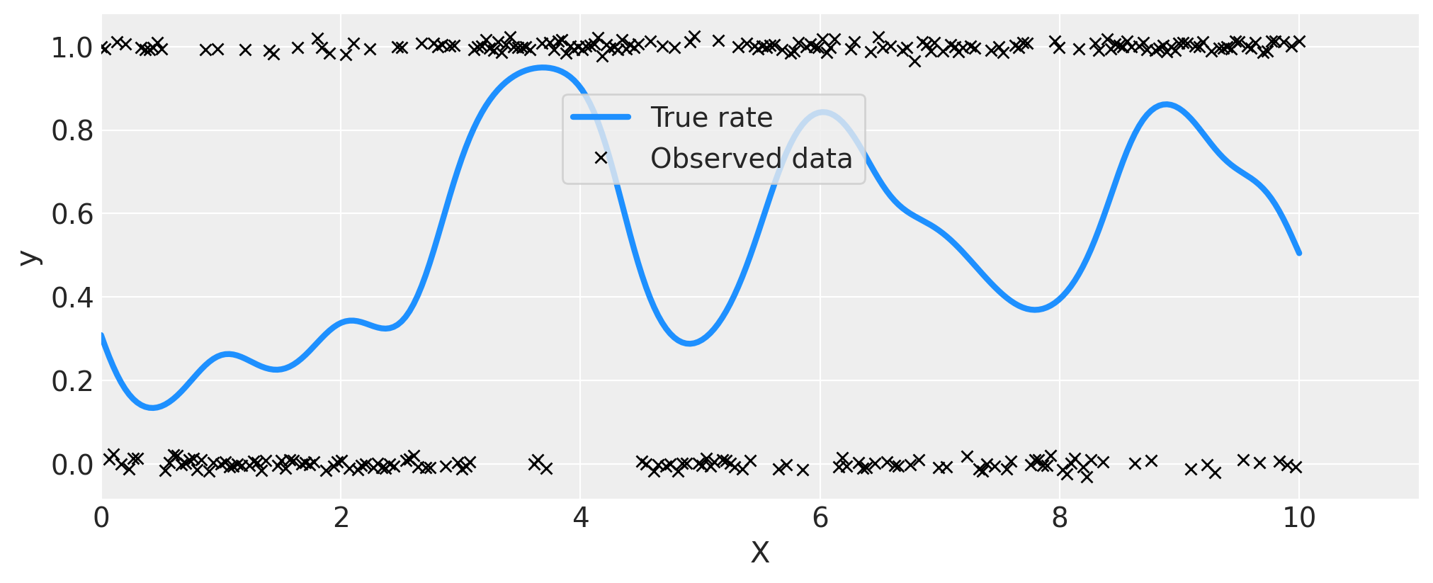
首先,我们使用 GP 生成一些遵循伯努利分布的数据,其中 \(p\),即获得 1 而不是 0 的概率是 \(x\) 的函数。我重置了种子并添加了更多伪造数据点,因为模型可能难以辨别 0.5 附近的变异,而观测值很少。
# reset the random seed for the new example
RANDOM_SEED = 8888
rng = np.random.default_rng(RANDOM_SEED)

# number of data points
n = 300

# x locations
x = np.linspace(0, 10, n)

# true covariance
ell_true = 0.5
eta_true = 1.0
cov_func = eta_true**2 * pm.gp.cov.ExpQuad(1, ell_true)
K = cov_func(x[:, None]).eval()

# zero mean function
mean = np.zeros(n)

# sample from the gp prior
f_true = pm.draw(pm.MvNormal.dist(mu=mean, cov=K), 1, random_seed=rng)

# Sample the GP through the likelihood
y = pm.Bernoulli.dist(p=pm.math.invlogit(f_true)).eval()
fig = plt.figure(figsize=(10, 4))
ax = fig.gca()

ax.plot(x, pm.math.invlogit(f_true).eval(), "dodgerblue", lw=3, label="True rate")
# add some noise to y to make the points in the plot more visible
ax.plot(x, y + np.random.randn(n) * 0.01, "kx", ms=6, label="Observed data")

ax.set_xlabel("X")
ax.set_ylabel("y")
ax.set_xlim([0, 11])
plt.legend(loc=(0.35, 0.65), frameon=True);
with pm.Model() as model:
    ell = pm.InverseGamma("ell", mu=1.0, sigma=0.5)
    eta = pm.Exponential("eta", lam=1.0)
    cov = eta**2 * pm.gp.cov.ExpQuad(1, ell)

    gp = pm.gp.Latent(cov_func=cov)
    f = gp.prior("f", X=x[:, None])

    # logit link and Bernoulli likelihood
    p = pm.Deterministic("p", pm.math.invlogit(f))
    y_ = pm.Bernoulli("y", p=p, observed=y)

    idata = pm.sample(1000, chains=2, cores=2, nuts_sampler="numpyro")
We recommend running at least 4 chains for robust computation of convergence diagnostics
# check Rhat, values above 1 may indicate convergence issues
n_nonconverged = int(np.sum(az.rhat(idata)[["eta", "ell", "f_rotated_"]].to_array() > 1.03).values)
if n_nonconverged == 0:
    print("No Rhat values above 1.03, \N{check mark}")
else:
    print(f"The MCMC chains for {n_nonconverged} RVs appear not to have converged.")
No Rhat values above 1.03, ✓
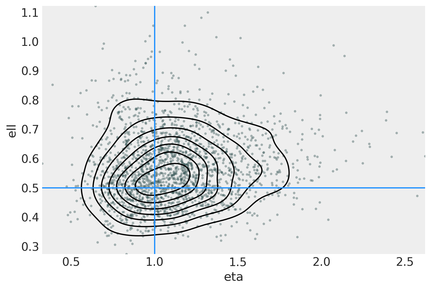
ax = az.plot_pair(
    idata,
    var_names=["eta", "ell"],
    kind=["kde", "scatter"],
    scatter_kwargs={"color": "darkslategray", "alpha": 0.4},
    gridsize=25,
    divergences=True,
)

ax.axvline(x=eta_true, color="dodgerblue")
ax.axhline(y=ell_true, color="dodgerblue");
n_pred = 200
X_new = np.linspace(0, 12, n_pred)[:, None]

with model:
    f_pred = gp.conditional("f_pred", X_new, jitter=1e-4)
    p_pred = pm.Deterministic("p_pred", pm.math.invlogit(f_pred))

with model:
    idata.extend(pm.sample_posterior_predictive(idata.posterior, var_names=["f_pred", "p_pred"]))
Sampling: [f_pred]
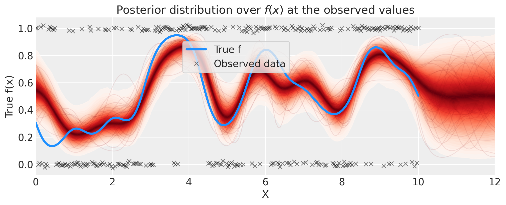
# plot the results
fig = plt.figure(figsize=(10, 4))
ax = fig.gca()

# plot the samples from the gp posterior with samples and shading
p_pred = az.extract(idata.posterior_predictive, var_names="p_pred").transpose("sample", ...)
plot_gp_dist(ax, p_pred, X_new)

# plot the data (with some jitter) and the true latent function
plt.plot(x, pm.math.invlogit(f_true).eval(), "dodgerblue", lw=3, label="True f")
plt.plot(
    x,
    y + np.random.randn(y.shape[0]) * 0.01,
    "kx",
    ms=6,
    alpha=0.5,
    label="Observed data",
)

# axis labels and title
plt.xlabel("X")
plt.ylabel("True f(x)")
plt.xlim([0, 12])
plt.title("Posterior distribution over $f(x)$ at the observed values")
plt.legend(loc=(0.32, 0.65), frameon=True);
水印#
%load_ext watermark
%watermark -n -u -v -iv -w -p pytensor,aeppl,xarray
Last updated: Mon May 27 2024

Python implementation: CPython
Python version       : 3.12.2
IPython version      : 8.22.2

pytensor: 2.20.0
aeppl   : not installed
xarray  : 2024.3.0

matplotlib: 3.8.3
numpy     : 1.26.4
pymc      : 5.15.0+14.gfd11cf012
arviz     : 0.17.1

Watermark: 2.4.3
许可声明#
此示例库中的所有笔记本均根据 MIT 许可证提供,该许可证允许修改和再分发以用于任何用途,前提是保留版权和许可声明。
引用 PyMC 示例#
要引用此笔记本,请使用 Zenodo 为 pymc-examples 存储库提供的 DOI。
重要提示
许多笔记本改编自其他来源:博客、书籍……在这种情况下,您也应该引用原始来源。
另请记住引用您的代码使用的相关库。
这是一个 bibtex 中的引用模板
@incollection{citekey,
  author    = "<notebook authors, see above>",
  title     = "<notebook title>",
  editor    = "PyMC Team",
  booktitle = "PyMC examples",
  doi       = "10.5281/zenodo.5654871"
}
渲染后可能如下所示