边缘似然实现#

gp.Marginal 类实现了 GP 回归更常见的情况：观测数据是 GP 和高斯噪声的总和。gp.Marginal 具有 marginal_likelihood 方法、conditional 方法和 predict 方法。给定均值和协方差函数，函数 \(f(x)\) 被建模为，

\[ f(x) \sim \mathcal{GP}(m(x),\, k(x, x')) \,. \]

观测值 \(y\) 是未知函数加上噪声

\[\begin{split} \begin{aligned} \epsilon &\sim N(0, \Sigma) \\ y &= f(x) + \epsilon \\ \end{aligned} \end{split}\]

`.marginal_likelihood` 方法#

未知的潜在函数可以从 GP 先验概率与正态似然的乘积中解析积分出来。这个量被称为边缘似然。

\[ p(y \mid x) = \int p(y \mid f, x) \, p(f \mid x) \, df \]

边缘似然的对数，\(p(y \mid x)\)，是

\[ \log p(y \mid x) = -\frac{1}{2} (\mathbf{y} - \mathbf{m}_x)^{T} (\mathbf{K}_{xx} + \boldsymbol\Sigma)^{-1} (\mathbf{y} - \mathbf{m}_x) - \frac{1}{2}\log(\mathbf{K}_{xx} + \boldsymbol\Sigma) - \frac{n}{2}\log (2 \pi) \]

\(\boldsymbol\Sigma\) 是高斯噪声的协方差矩阵。由于高斯噪声不需要是白噪声才能共轭，因此当提供标量时，marginal_likelihood 方法支持使用白噪声项，或者当提供协方差函数时，支持使用噪声协方差函数。

gp.marginal_likelihood 方法实现了上面给出的量。一些示例代码如下，

import numpy as np
import pymc3 as pm

# A one dimensional column vector of inputs.
X = np.linspace(0, 1, 10)[:,None]

with pm.Model() as marginal_gp_model:
    # Specify the covariance function.
    cov_func = pm.gp.cov.ExpQuad(1, ls=0.1)

    # Specify the GP.  The default mean function is `Zero`.
    gp = pm.gp.Marginal(cov_func=cov_func)

    # The scale of the white noise term can be provided,
    sigma = pm.HalfCauchy("sigma", beta=5)
    y_ = gp.marginal_likelihood("y", X=X, y=y, sigma=sigma)
    
    # OR a covariance function for the noise can be given
    # noise_l = pm.Gamma("noise_l", alpha=2, beta=2)
    # cov_func_noise = pm.gp.cov.Exponential(1, noise_l) + pm.gp.cov.WhiteNoise(sigma=0.1)
    # y_ = gp.marginal_likelihood("y", X=X, y=y, sigma=cov_func_noise)

`.conditional` 分布#

.conditional 有一个可选标志 pred_noise，默认为 False。当 pred_sigma=False 时，conditional 方法生成 GP 表示的底层函数的预测分布。当 pred_sigma=True 时，conditional 方法生成 GP 加噪声的预测分布。使用上面定义的相同 gp 对象，

# vector of new X points we want to predict the function at
Xnew = np.linspace(0, 2, 100)[:, None]

with marginal_gp_model:
    f_star = gp.conditional("f_star", Xnew=Xnew)
    
    # or to predict the GP plus noise
    y_star = gp.conditional("y_star", Xnew=Xnew, pred_sigma=True)

如果使用加性 GP 模型，可以通过设置可选参数 given 来构建各个分量的条件分布。有关构建加性 GP 的更多信息，请参阅主文档页面。有关示例，请参阅 Mauna Loa CO\(_2\) 笔记本。

进行预测#

.predict 方法返回给定 point 的 gp 的条件均值和方差作为 NumPy 数组。point 可以是 find_MAP 的结果或来自迹的样本。.predict 方法可以在 Model 块外部使用。与 .conditional 类似，.predict 接受 given，因此它可以从加性 GP 的分量生成预测。

# The mean and full covariance
mu, cov = gp.predict(Xnew, point=trace[-1])

# The mean and variance (diagonal of the covariance)
mu, var = gp.predict(Xnew, point=trace[-1],  diag=True)

# With noise included
mu, var = gp.predict(Xnew, point=trace[-1],  diag=True, pred_sigma=True)

示例：使用白色高斯噪声进行回归#

import arviz as az
import matplotlib.pyplot as plt
import numpy as np
import pandas as pd
import pymc as pm
import scipy as sp

%matplotlib inline

# set the seed
np.random.seed(1)

n = 100  # The number of data points
X = np.linspace(0, 10, n)[:, None]  # The inputs to the GP, they must be arranged as a column vector

# Define the true covariance function and its parameters
ell_true = 1.0
eta_true = 3.0
cov_func = eta_true**2 * pm.gp.cov.Matern52(1, ell_true)

# A mean function that is zero everywhere
mean_func = pm.gp.mean.Zero()

# The latent function values are one sample from a multivariate normal
# Note that we have to call `eval()` because PyMC3 built on top of Theano
f_true = np.random.multivariate_normal(
    mean_func(X).eval(), cov_func(X).eval() + 1e-8 * np.eye(n), 1
).flatten()

# The observed data is the latent function plus a small amount of IID Gaussian noise
# The standard deviation of the noise is `sigma`
sigma_true = 2.0
y = f_true + sigma_true * np.random.randn(n)

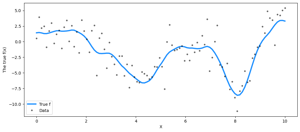
## Plot the data and the unobserved latent function
fig = plt.figure(figsize=(12, 5))
ax = fig.gca()
ax.plot(X, f_true, "dodgerblue", lw=3, label="True f")
ax.plot(X, y, "ok", ms=3, alpha=0.5, label="Data")
ax.set_xlabel("X")
ax.set_ylabel("The true f(x)")
plt.legend();

../_images/2447e8ebbc842686109ae1c94a562490c64513eb6923e57e310fd86563d08d66.png

with pm.Model() as model:
    ell = pm.Gamma("ell", alpha=2, beta=1)
    eta = pm.HalfCauchy("eta", beta=5)

    cov = eta**2 * pm.gp.cov.Matern52(1, ell)
    gp = pm.gp.Marginal(cov_func=cov)

    sigma = pm.HalfCauchy("sigma", beta=5)
    y_ = gp.marginal_likelihood("y", X=X, y=y, sigma=sigma)

    with model:
        marginal_post = pm.sample(500, tune=2000, nuts_sampler="numpyro", chains=1)

/Users/cfonnesbeck/mambaforge/envs/bayes_course/lib/python3.11/site-packages/pymc/sampling/mcmc.py:243: UserWarning: Use of external NUTS sampler is still experimental
  warnings.warn("Use of external NUTS sampler is still experimental", UserWarning)

Compiling...
Compilation time =  0:00:00.634832
Sampling...

sample: 100%|██████████| 2500/2500 [00:20<00:00, 119.94it/s, 7 steps of size 5.25e-01. acc. prob=0.92] 

Sampling time =  0:00:23.334210
Transforming variables...
Transformation time =  0:00:00.014305

summary = az.summary(marginal_post, var_names=["ell", "eta", "sigma"], round_to=2, kind="stats")
summary["True value"] = [ell_true, eta_true, sigma_true]
summary

	均值	标准差	hdi_3%	hdi_97%	真实值
ell	1.18	0.28	0.72	1.76	1.0
eta	4.39	1.30	2.67	7.09	3.0
sigma	1.93	0.14	1.68	2.20	2.0

估计值接近它们的真实值。

使用 `.conditional`#

# new values from x=0 to x=20
X_new = np.linspace(0, 20, 600)[:, None]

# add the GP conditional to the model, given the new X values
with model:
    f_pred = gp.conditional("f_pred", X_new)

with model:
    pred_samples = pm.sample_posterior_predictive(
        marginal_post.sel(draw=slice(0, 20)), var_names=["f_pred"]
    )

Sampling: [f_pred]

100.00% [21/21 00:56<00:00]

# plot the results
fig = plt.figure(figsize=(12, 5))
ax = fig.gca()

# plot the samples from the gp posterior with samples and shading
from pymc.gp.util import plot_gp_dist

f_pred_samples = az.extract(pred_samples, group="posterior_predictive", var_names=["f_pred"])
plot_gp_dist(ax, samples=f_pred_samples.T, x=X_new)

# plot the data and the true latent function
plt.plot(X, f_true, "dodgerblue", lw=3, label="True f")
plt.plot(X, y, "ok", ms=3, alpha=0.5, label="Observed data")

# axis labels and title
plt.xlabel("X")
plt.ylim([-13, 13])
plt.title("Posterior distribution over $f(x)$ at the observed values")
plt.legend();

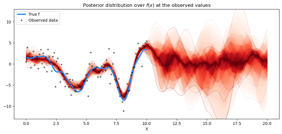
../_images/99733747e5afbc6acc61db1deecb5fe806a311fef683e5d39e6ad642ce73cc1b.png

预测也与 gp.Latent 的结果非常吻合。预测新数据点怎么样？这里我们只预测了 \(f_*\)，而不是 \(f_*\) + 噪声，这才是我们实际观察到的。

gp.Marginal 的 conditional 方法包含标志 pred_noise，其默认值为 False。要从后验预测分布中抽样，我们只需将此标志设置为 True。

with model:
    y_pred = gp.conditional("y_pred", X_new, pred_noise=True)
    y_samples = pm.sample_posterior_predictive(
        marginal_post.sel(draw=slice(0, 50)), var_names=["y_pred"]
    )

Sampling: [y_pred]

100.00% [51/51 01:19<00:00]

fig = plt.figure(figsize=(12, 5))
ax = fig.gca()

# posterior predictive distribution
y_pred_samples = az.extract(y_samples, group="posterior_predictive", var_names=["y_pred"])
plot_gp_dist(ax, y_pred_samples.T, X_new, plot_samples=False, palette="bone_r")

# overlay a scatter of one draw of random points from the
#   posterior predictive distribution
plt.plot(X_new, y_pred_samples.sel(sample=1), "co", ms=2, label="Predicted data")

# plot original data and true function
plt.plot(X, y, "ok", ms=3, alpha=1.0, label="observed data")
plt.plot(X, f_true, "dodgerblue", lw=3, label="true f")

plt.xlabel("x")
plt.ylim([-13, 13])
plt.title("posterior predictive distribution, y_*")
plt.legend();

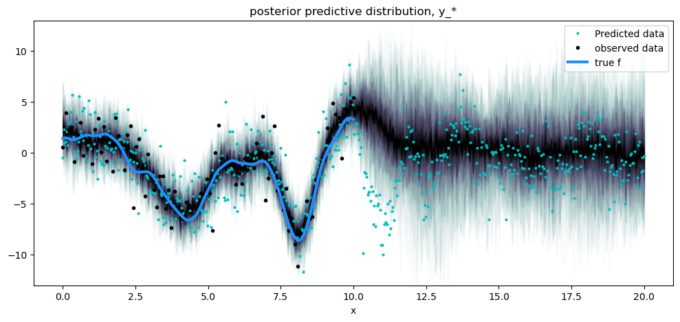
../_images/d3330db4a453e459d7141bbd2bbb73c35ad884c3a43d0f1aea92f61623917071.png

请注意，后验预测密度比无噪声函数的条件分布更宽，并反映了噪声数据的预测分布，标记为黑点。浅色点并不完全遵循预测密度的扩散，因为它们是从 GP 加噪声的后验中抽取的一个样本。

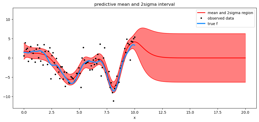
使用 `.predict`#

我们可以使用 .predict 方法返回给定特定 point 的均值和方差。

# predict
with model:
    mu, var = gp.predict(
        X_new, point=az.extract(marginal_post.posterior.sel(draw=[0])).squeeze(), diag=True
    )
sd = np.sqrt(var)

# draw plot
fig = plt.figure(figsize=(12, 5))
ax = fig.gca()

# plot mean and 2sigma intervals
plt.plot(X_new, mu, "r", lw=2, label="mean and 2σ region")
plt.plot(X_new, mu + 2 * sd, "r", lw=1)
plt.plot(X_new, mu - 2 * sd, "r", lw=1)
plt.fill_between(X_new.flatten(), mu - 2 * sd, mu + 2 * sd, color="r", alpha=0.5)

# plot original data and true function
plt.plot(X, y, "ok", ms=3, alpha=1.0, label="observed data")
plt.plot(X, f_true, "dodgerblue", lw=3, label="true f")

plt.xlabel("x")
plt.ylim([-13, 13])
plt.title("predictive mean and 2sigma interval")
plt.legend();

../_images/9d1295be5bbc6b6911dd5280f3161ded6974f82792055d55648bd4df7fea9a1e.png

作者#

由 Bill Engels 于 2017 年创建 (pymc#1674)
由 Colin Caroll 于 2019 年重新执行 (pymc#3397)
由 Bill Engels 于 2022 年 9 月更新为 V4 版本 (pymc-examples#237)
由 Chris Fonnesbeck 于 2023 年 7 月更新为 V5 版本 (pymc-examples#549)

水印#

%load_ext watermark
%watermark -n -u -v -iv -w

Last updated: Mon Jun 05 2023

Python implementation: CPython
Python version       : 3.11.3
IPython version      : 8.13.2

arviz     : 0.15.1
scipy     : 1.10.1
pymc      : 5.3.0
pandas    : 2.0.2
numpy     : 1.24.3
matplotlib: 3.7.1

Watermark: 2.3.1

分类

标签

边缘似然实现#

`.marginal_likelihood` 方法#

`.conditional` 分布#

进行预测#

示例：使用白色高斯噪声进行回归#

使用 `.conditional`#

使用 `.predict`#

作者#

水印#

分类

标签

边缘似然实现#

.marginal_likelihood 方法#

.conditional 分布#

进行预测#

示例：使用白色高斯噪声进行回归#

使用 .conditional#

使用 .predict#

作者#

水印#

`.marginal_likelihood` 方法#

`.conditional` 分布#

使用 `.conditional`#

使用 `.predict`#