Student-t 过程

PyMC 也包括 T 过程先验。它们是将高斯过程先验推广到多元 Student’s T 分布。用法与 gp.Latent 相同，除了在模型中指定时，它们需要自由度参数。有关更多信息，请参阅 Rasmussen+Williams 的第 9 章和 Shah et al.。

请注意，T 过程的加法性与 GP 不同，因此不支持添加 TP 对象。

TP 先验的样本

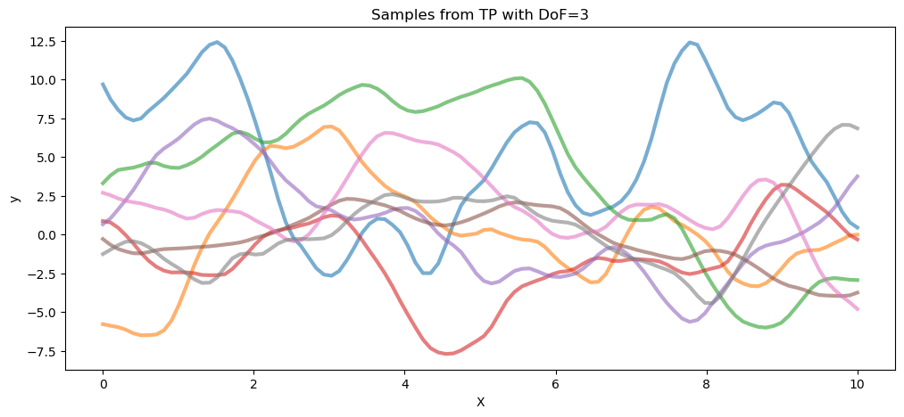
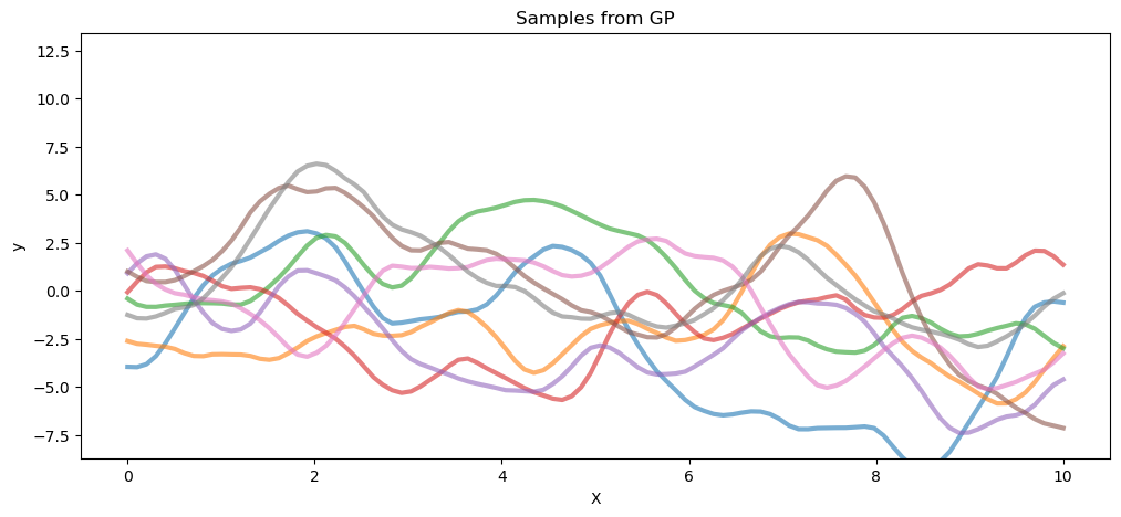
以下代码从自由度为 3 的 T 过程先验和高斯过程（两者都具有相同的协方差矩阵）中抽取样本。

import arviz as az
import matplotlib.pyplot as plt
import numpy as np
import pymc as pm
import pytensor.tensor as pt

from pymc.gp.util import plot_gp_dist

%matplotlib inline

# set the seed
np.random.seed(1)

n = 100  # The number of data points
X = np.linspace(0, 10, n)[:, None]  # The inputs to the GP, they must be arranged as a column vector

# Define the true covariance function and its parameters
ell_true = 1.0
eta_true = 3.0
cov_func = eta_true**2 * pm.gp.cov.Matern52(1, ell_true)

# A mean function that is zero everywhere
mean_func = pm.gp.mean.Zero()

# The latent function values are one sample from a multivariate normal
# Note that we have to call `eval()` because PyMC3 built on top of Theano
tp_samples = pm.draw(pm.MvStudentT.dist(mu=mean_func(X).eval(), scale=cov_func(X).eval(), nu=3), 8)

## Plot samples from TP prior
fig = plt.figure(figsize=(12, 5))
ax0 = fig.gca()
ax0.plot(X.flatten(), tp_samples.T, lw=3, alpha=0.6)
ax0.set_xlabel("X")
ax0.set_ylabel("y")
ax0.set_title("Samples from TP with DoF=3")


gp_samples = pm.draw(pm.MvNormal.dist(mu=mean_func(X).eval(), cov=cov_func(X).eval()), 8)
fig = plt.figure(figsize=(12, 5))
ax1 = fig.gca()
ax1.plot(X.flatten(), gp_samples.T, lw=3, alpha=0.6)
ax1.set_xlabel("X")
ax1.set_ylabel("y")
ax1.set_ylim(ax0.get_ylim())
ax1.set_title("Samples from GP");

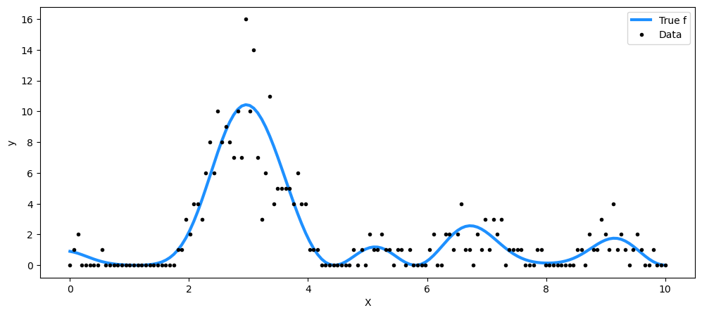
由 T 过程生成的泊松数据

对于泊松率，我们取 T 过程先验表示的函数的平方。

np.random.seed(7)

n = 150  # The number of data points
X = np.linspace(0, 10, n)[:, None]  # The inputs to the GP, they must be arranged as a column vector

# Define the true covariance function and its parameters
ell_true = 1.0
eta_true = 3.0
cov_func = eta_true**2 * pm.gp.cov.ExpQuad(1, ell_true)

# A mean function that is zero everywhere
mean_func = pm.gp.mean.Zero()

# The latent function values are one sample from a multivariate normal
# Note that we have to call `eval()` because PyMC3 built on top of Theano
f_true = pm.draw(pm.MvStudentT.dist(mu=mean_func(X).eval(), scale=cov_func(X).eval(), nu=3), 1)
y = np.random.poisson(f_true**2)

fig = plt.figure(figsize=(12, 5))
ax = fig.gca()
ax.plot(X, f_true**2, "dodgerblue", lw=3, label="True f")
ax.plot(X, y, "ok", ms=3, label="Data")
ax.set_xlabel("X")
ax.set_ylabel("y")
plt.legend();

with pm.Model() as model:
    ell = pm.Gamma("ell", alpha=2, beta=2)
    eta = pm.HalfCauchy("eta", beta=3)
    cov = eta**2 * pm.gp.cov.ExpQuad(1, ell)

    # informative prior on degrees of freedom < 5
    nu = pm.Gamma("nu", alpha=2, beta=1)
    tp = pm.gp.TP(scale_func=cov, nu=nu)
    f = tp.prior("f", X=X)

    pm.Poisson("y", mu=pt.square(f), observed=y)

    tr = pm.sample(target_accept=0.9, nuts_sampler="nutpie", chains=2)

/var/home/fonnesbeck/repos/pymc-examples/.pixi/envs/default/lib/python3.12/site-packages/pytensor/graph/rewriting/basic.py:121: UserWarning: A Supervisor feature is missing from FunctionGraph(AdvancedSetSubtensor(Alloc(0.0, *2 -> Shape_i{0}(*0-<Vector(float64, shape=(?,))>), *2), *0-<Vector(float64, shape=(?,))>, *1 -> ARange{dtype='int64'}(0, *2, 1), *1)).
  return self.apply(fgraph, *args, **kwargs)
/var/home/fonnesbeck/repos/pymc-examples/.pixi/envs/default/lib/python3.12/site-packages/pytensor/link/numba/dispatch/basic.py:377: UserWarning: Numba will use object mode to run AdvancedSetSubtensor's perform method
  warnings.warn(
/var/home/fonnesbeck/repos/pymc-examples/.pixi/envs/default/lib/python3.12/site-packages/pytensor/graph/rewriting/basic.py:121: UserWarning: A Supervisor feature is missing from FunctionGraph(AdvancedSetSubtensor(Alloc(0.0, *1 -> Shape_i{0}(*0-<Vector(float64, shape=(?,))>), *1), *0-<Vector(float64, shape=(?,))>, *2 -> ARange{dtype='int64'}(0, *1, 1), *2)).
  return self.apply(fgraph, *args, **kwargs)
/var/home/fonnesbeck/repos/pymc-examples/.pixi/envs/default/lib/python3.12/site-packages/pytensor/link/numba/dispatch/basic.py:377: UserWarning: Numba will use object mode to run AdvancedSetSubtensor's perform method
  warnings.warn(

采样器进度

总链数：2

活动链数：0

已完成链数：2

采样 4 分钟

预计完成时间：now

进度	抽取	发散	步长	梯度/抽取
	2000	21	0.07	127
	2000	13	0.08	127

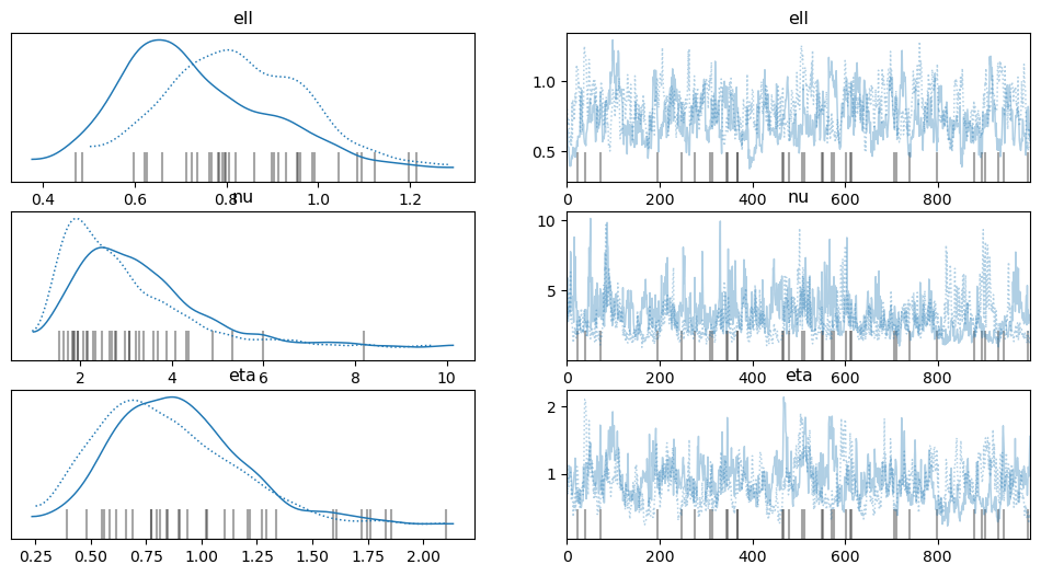
az.plot_trace(tr, var_names=["ell", "nu", "eta"]);

n_new = 200
X_new = np.linspace(0, 15, n_new)[:, None]

# add the GP conditional to the model, given the new X values
with model:
    f_pred = tp.conditional("f_pred", X_new)

# Sample from the GP conditional distribution
with model:
    pm.sample_posterior_predictive(tr, var_names=["f_pred"], extend_inferencedata=True)

Sampling: [f_pred]

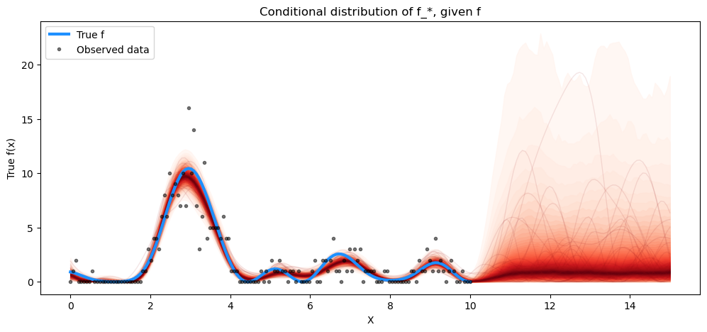
fig = plt.figure(figsize=(12, 5))
ax = fig.gca()

f_pred_samples = np.square(
    az.extract(tr.posterior_predictive).astype(np.float32)["f_pred"].values
).T
plot_gp_dist(ax, f_pred_samples, X_new)
plt.plot(X, np.square(f_true), "dodgerblue", lw=3, label="True f")
plt.plot(X, y, "ok", ms=3, alpha=0.5, label="Observed data")
plt.xlabel("X")
plt.ylabel("True f(x)")
plt.title("Conditional distribution of f_*, given f")
plt.legend();

作者

• 作者：Bill Engels

• 更新者：Chris Fonnesbeck，使用 PyMC v5

参考文献

%load_ext watermark
%watermark -n -u -v -iv -w

Last updated: Fri Sep 20 2024

Python implementation: CPython
Python version       : 3.12.5
IPython version      : 8.27.0

matplotlib: 3.9.2
arviz     : 0.19.0
numpy     : 1.26.4
pymc      : 5.16.2
pytensor  : 2.25.4

Watermark: 2.4.3