


二项回归#
本笔记本涵盖了二项回归背后的逻辑,它是广义线性建模的一个特定实例。示例非常简单,只有一个预测变量。
为了理解何时适用二项回归,回顾逻辑回归会有所帮助。当你的结果变量是一系列成功或失败,即一系列 0、1 观测值时,逻辑回归非常有用。这种结果变量的一个例子是“你今天去跑步了吗?”。当你有一定数量的成功次数(在 \(n\) 次试验中)时,二项回归(也称为聚合二项回归)非常有用。因此,示例将是“过去 7 天你跑了多少天?”
观测数据是一组在 \(n\) 次总试验中成功的计数。 许多人可能倾向于将此数据简化为比例,但这不一定是好主意。 例如,比例不是直接测量的,它们通常最好被视为要估计的潜在变量。 此外,比例会丢失信息:0.5 的比例可能对应于 2 天中跑 1 次,或者过去 4 周中跑 4 次,或者许多其他情况,但你已经通过仅关注比例而丢失了该信息。
二项回归的适当似然函数是二项分布
其中 \(y_i\) 是 \(n\) 次试验中成功次数的计数,而 \(p_i\) 是(潜在的)成功概率。 二项回归想要实现的目标是使用线性模型来准确估计 \(p_i\)(即 \(p_i = \beta_0 + \beta_1 \cdot x_i\))。 因此,我们可以尝试使用如下似然项来做到这一点
如果我们这样做,当线性模型生成 \(p\) 值超出 \(0-1\) 范围时,我们将很快遇到问题。 这就是链接函数发挥作用的地方
其中 \(g()\) 是链接函数。 这可以被认为是将 \((0, 1)\) 范围内的比例映射到 \((-\infty, +\infty)\) 域的转换。 有许多潜在的函数可以使用,但常用的函数是 Logit 函数。
虽然我们实际想要做的是为 \(p_i\) 重新排列此方程,以便我们可以将其输入到似然函数中。 这导致
其中 \(g^{-1}()\) 是链接函数的逆函数,在本例中是 Logit 函数的逆函数(即 logistic sigmoid 函数,也称为 expit 函数)。 因此,如果我们将其输入到我们的似然函数中,我们最终得到
这定义了我们的似然函数。 现在,要完成一些贝叶斯二项回归,你只需要 \(\beta\) 参数的先验。 观测数据是 \(y_i\)、\(n\) 和 \(x_i\)。
import arviz as az
import matplotlib.pyplot as plt
import numpy as np
import pandas as pd
import pymc as pm

from scipy.special import expit
%config InlineBackend.figure_format = 'retina'
az.style.use("arviz-darkgrid")
rng = np.random.default_rng(1234)
生成数据#
# true params
beta0_true = 0.7
beta1_true = 0.4
# number of yes/no questions
n = 20

sample_size = 30
x = np.linspace(-10, 20, sample_size)
# Linear model
mu_true = beta0_true + beta1_true * x
# transformation (inverse logit function = expit)
p_true = expit(mu_true)
# Generate data
y = rng.binomial(n, p_true)
# bundle data into dataframe
data = pd.DataFrame({"x": x, "y": y})
我们可以看到,底层数据 \(y\) 是计数数据,在 \(n\) 次总试验中。
data.head()
| x | y | |
|---|---|---|
| 0 | -10.000000 | 3 |
| 1 | -8.965517 | 1 |
| 2 | -7.931034 | 3 |
| 3 | -6.896552 | 1 |
| 4 | -5.862069 | 2 |
显示代码单元格源
# Plot underlying linear model
fig, ax = plt.subplots(2, 1, figsize=(9, 6), sharex=True)
ax[0].plot(x, mu_true, label=r"$β_0 + β_1 \cdot x_i$")
ax[0].set(xlabel="$x$", ylabel=r"$β_0 + β_1 \cdot x_i$", title="Underlying linear model")
ax[0].legend()

# Plot GLM
freq = ax[1].twinx()  # instantiate a second axes that shares the same x-axis
freq.set_ylabel("number of successes")
freq.scatter(x, y, color="k")
# plot proportion related stuff on ax[1]
ax[1].plot(x, p_true, label=r"$g^{-1}(β_0 + β_1 \cdot x_i)$")
ax[1].set_ylabel("proportion successes", color="b")
ax[1].tick_params(axis="y", labelcolor="b")
ax[1].set(xlabel="$x$", title="Binomial regression")
ax[1].legend()
# get y-axes to line up
y_buffer = 1
freq.set(ylim=[-y_buffer, n + y_buffer])
ax[1].set(ylim=[-(y_buffer / n), 1 + (y_buffer / n)])
freq.grid(None)
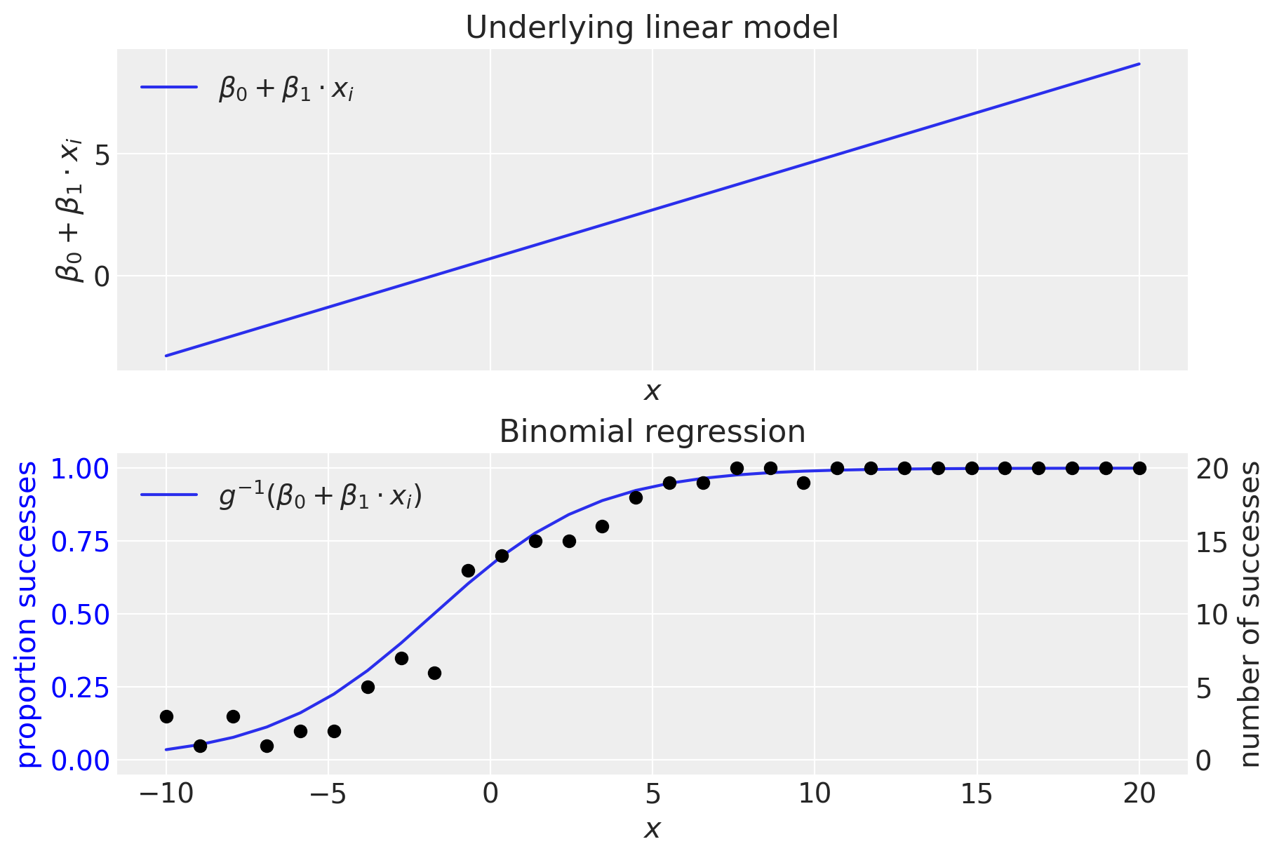
顶部面板显示(未转换的)线性模型。 我们可以看到,线性模型正在生成超出 \(0-1\) 范围的值,这清楚地表明需要逆链接函数 \(g^{-1}()\),它从 \((-\infty, +\infty) \rightarrow (0, 1)\) 域进行转换。 正如我们所见,这是通过逆逻辑函数(又名逻辑 sigmoid 函数)完成的。
二项回归模型#
从技术上讲,我们不需要提供 coords,但提供此项(观测值列表)有助于稍后重塑数据数组。 coords 中的信息由模型中的 dims kwarg 使用。
coords = {"observation": data.index.values}

with pm.Model(coords=coords) as binomial_regression_model:
    x = pm.ConstantData("x", data["x"], dims="observation")
    # priors
    beta0 = pm.Normal("beta0", mu=0, sigma=1)
    beta1 = pm.Normal("beta1", mu=0, sigma=1)
    # linear model
    mu = beta0 + beta1 * x
    p = pm.Deterministic("p", pm.math.invlogit(mu), dims="observation")
    # likelihood
    pm.Binomial("y", n=n, p=p, observed=data["y"], dims="observation")
pm.model_to_graphviz(binomial_regression_model)

with binomial_regression_model:
    idata = pm.sample(1000, tune=2000)
Sampling 4 chains for 2_000 tune and 1_000 draw iterations (8_000 + 4_000 draws total) took 1 seconds.
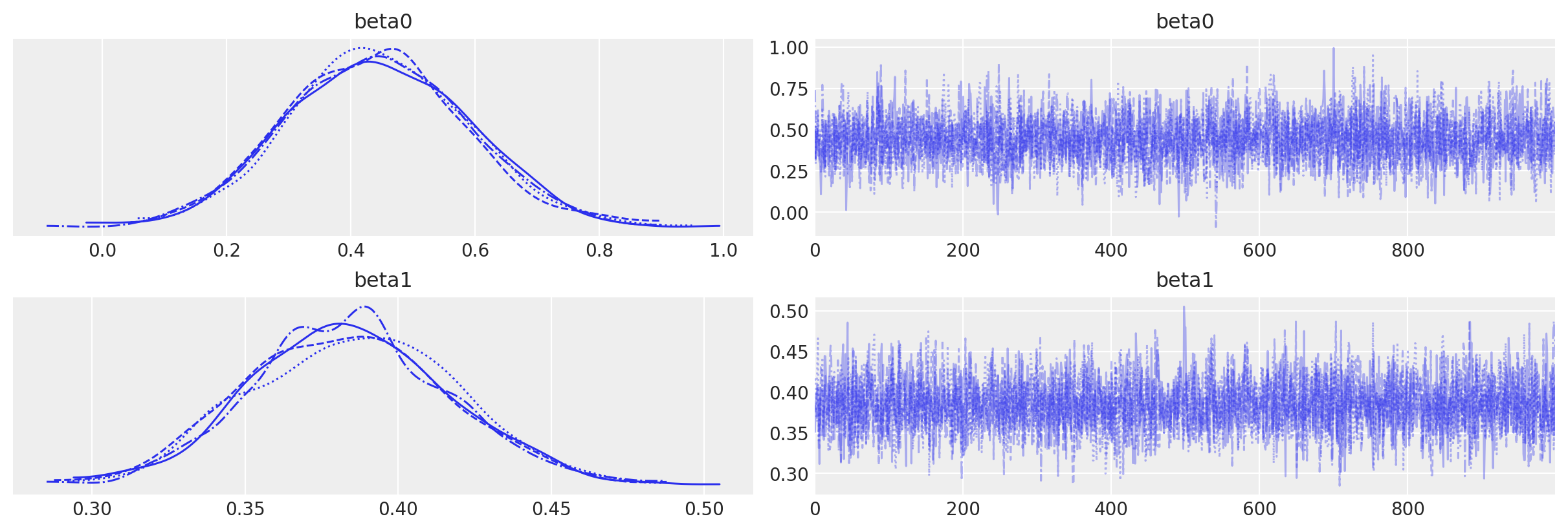
通过目视检查链来确认没有推断问题。 我们没有收到关于发散、\(\hat{R}\) 或有效样本量的警告。 一切看起来都很好。
az.plot_trace(idata, var_names=["beta0", "beta1"]);
检查结果#
下面的代码在数据空间中绘制模型预测,并在参数空间中绘制我们的后验信念。
显示代码单元格源
fig, ax = plt.subplots(1, 2, figsize=(9, 4), gridspec_kw={"width_ratios": [2, 1]})

# Data space plot ========================================================
az.plot_hdi(
    data["x"],
    idata.posterior.p,
    hdi_prob=0.95,
    fill_kwargs={"alpha": 0.25, "linewidth": 0},
    ax=ax[0],
    color="C1",
)
# posterior mean
post_mean = idata.posterior.p.mean(("chain", "draw"))
ax[0].plot(data["x"], post_mean, label="posterior mean", color="C1")
# plot truth
ax[0].plot(data["x"], p_true, "--", label="true", color="C2")
# formatting
ax[0].set(xlabel="x", title="Data space")
ax[0].set_ylabel("proportion successes", color="C1")
ax[0].tick_params(axis="y", labelcolor="C1")
ax[0].legend()
# instantiate a second axes that shares the same x-axis
freq = ax[0].twinx()
freq.set_ylabel("number of successes")
freq.scatter(data["x"], data["y"], color="k", label="data")
# get y-axes to line up
y_buffer = 1
freq.set(ylim=[-y_buffer, n + y_buffer])
ax[0].set(ylim=[-(y_buffer / n), 1 + (y_buffer / n)])
freq.grid(None)
# set both y-axis to have 5 ticks
ax[0].set(yticks=np.linspace(0, 20, 5) / n)
freq.set(yticks=np.linspace(0, 20, 5))

# Parameter space plot ===================================================
az.plot_kde(
    az.extract(idata, var_names="beta0"),
    az.extract(idata, var_names="beta1"),
    contourf_kwargs={"cmap": "Blues"},
    ax=ax[1],
)
ax[1].plot(beta0_true, beta1_true, "C2o", label="true")
ax[1].set(xlabel=r"$\beta_0$", ylabel=r"$\beta_1$", title="Parameter space")
ax[1].legend(facecolor="white", frameon=True);
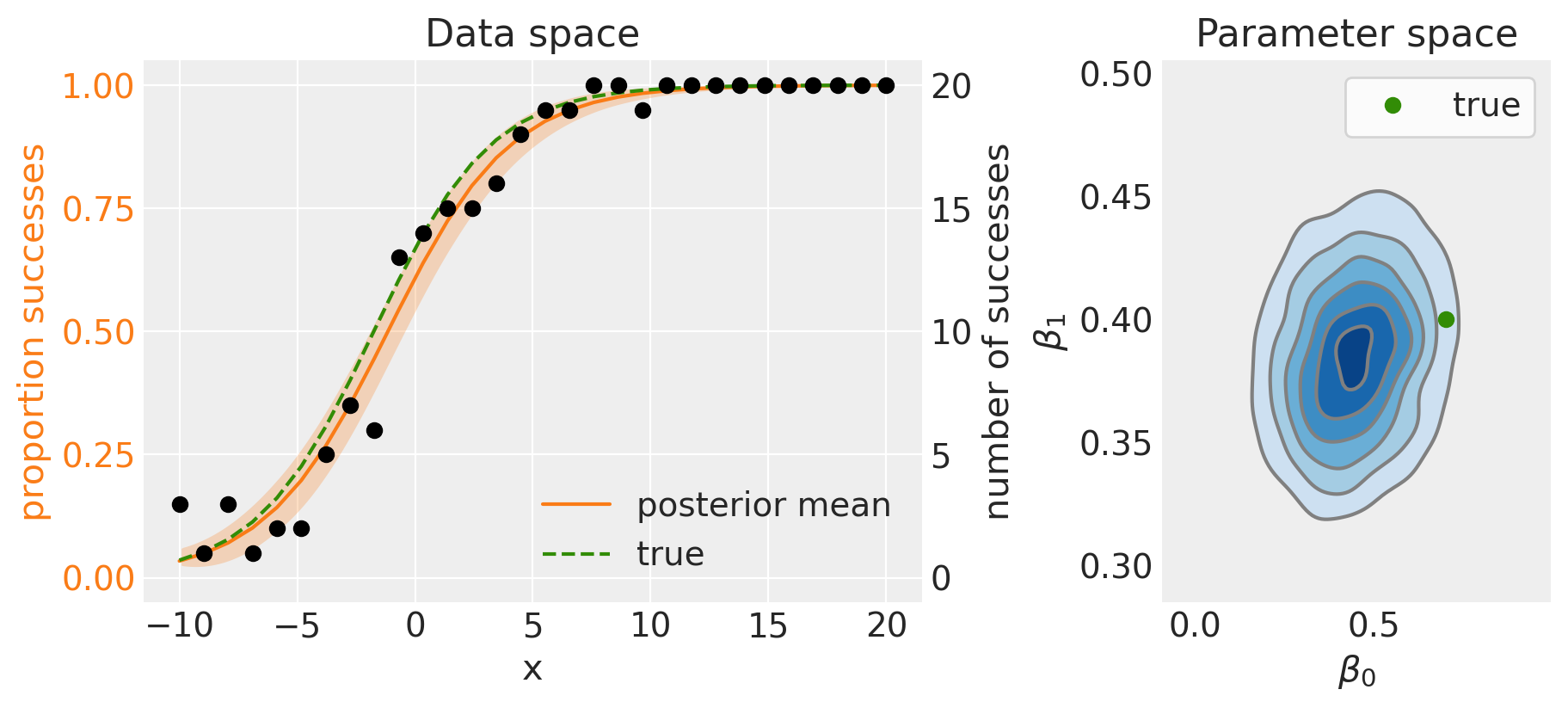
左侧面板显示后验均值(实线)和 95% 可信区间(阴影区域)。 因为我们正在使用模拟数据,所以我们知道真实模型是什么,因此我们可以看到后验均值与真实数据生成模型相比表现良好。
参数空间(右侧面板)上的后验分布也显示了这一点,当与真实数据生成参数进行比较时,它表现良好。
在实际数据分析情况下使用二项回归可能涉及更多的预测变量,以及相应更多的模型参数,但希望这个例子已经演示了二项回归背后的逻辑。
参考文献#
Roback, P. 和 J. Legler. 超越多元线性回归:R 中的应用广义线性模型和多层模型. CRC Press, 2021. URL: https://bookdown.org/roback/bookdown-BeyondMLR/.
水印#
%load_ext watermark
%watermark -n -u -v -iv -w -p pytensor,aeppl
Last updated: Sun Feb 05 2023

Python implementation: CPython
Python version       : 3.10.9
IPython version      : 8.9.0

pytensor: 2.8.11
aeppl   : not installed

matplotlib: 3.6.3
numpy     : 1.24.1
arviz     : 0.14.0
pandas    : 1.5.3
pymc      : 5.0.1

Watermark: 2.3.1