LKJ Cholesky 协方差先验用于多元正态模型#
虽然 逆 Wishart 分布 是多元正态分布协方差矩阵的共轭先验,但它不太适合现代贝叶斯计算方法。因此,在对多元正态分布的协方差矩阵进行建模时,建议使用 LKJ 先验。
为了说明使用 LKJ 分布对协方差进行建模,我们首先生成一个二维正态分布的样本数据集。
import arviz as az
import numpy as np
import pymc as pm

from matplotlib import pyplot as plt
from matplotlib.lines import Line2D
from matplotlib.patches import Ellipse

print(f"Running on PyMC v{pm.__version__}")
Running on PyMC v5.9.0
%config InlineBackend.figure_format = 'retina'
RANDOM_SEED = 8927
rng = np.random.default_rng(RANDOM_SEED)
az.style.use("arviz-darkgrid")
N = 10000

mu_actual = np.array([1.0, -2.0])
sigmas_actual = np.array([0.7, 1.5])
Rho_actual = np.matrix([[1.0, -0.4], [-0.4, 1.0]])

Sigma_actual = np.diag(sigmas_actual) * Rho_actual * np.diag(sigmas_actual)

x = rng.multivariate_normal(mu_actual, Sigma_actual, size=N)
Sigma_actual
matrix([[ 0.49, -0.42],
        [-0.42,  2.25]])
var, U = np.linalg.eig(Sigma_actual)
angle = 180.0 / np.pi * np.arccos(np.abs(U[0, 0]))

fig, ax = plt.subplots(figsize=(8, 6))

e = Ellipse(mu_actual, 2 * np.sqrt(5.991 * var[0]), 2 * np.sqrt(5.991 * var[1]), angle=angle)
e.set_alpha(0.5)
e.set_facecolor("C0")
e.set_zorder(10)
ax.add_artist(e)

ax.scatter(x[:, 0], x[:, 1], c="k", alpha=0.05, zorder=11)
ax.set_xlabel("y")
ax.set_ylabel("z")

rect = plt.Rectangle((0, 0), 1, 1, fc="C0", alpha=0.5)
ax.legend([rect], ["95% density region"], loc=2);
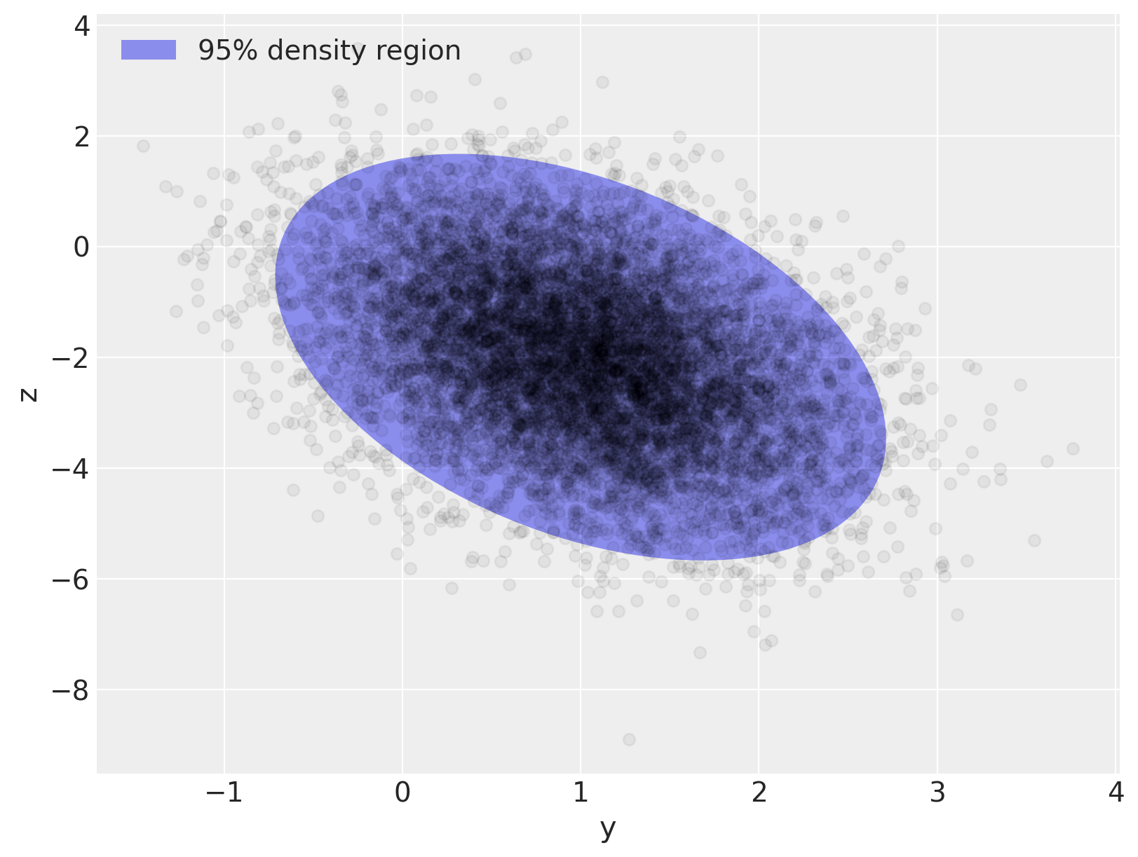
多元正态模型的抽样分布为 \(\mathbf{x} \sim N(\mu, \Sigma)\),其中 \(\Sigma\) 是抽样分布的协方差矩阵,且 \(\Sigma_{ij} = \textrm{Cov}(x_i, x_j)\)。此分布的密度为
LKJ 分布提供了相关矩阵的先验,\(\mathbf{C} = \textrm{Corr}(x_i, x_j)\),它与每个分量的标准差的先验相结合,导出协方差矩阵的先验,\(\Sigma\)。由于求逆 \(\Sigma\) 在数值上不稳定且效率低下,因此在计算上更有利的是使用 Cholesky 分解 \(\Sigma\),\(\Sigma = \mathbf{L} \mathbf{L}^{\top}\),其中 \(\mathbf{L}\) 是下三角矩阵。这种分解允许使用反向替换计算项 \((\mathbf{x} - \mu)^{\top} \Sigma^{-1} (\mathbf{x} - \mu)\),这比直接矩阵求逆在数值上更稳定和高效。
PyMC 通过 pymc.LKJCholeskyCov 分布支持协方差矩阵 Cholesky 分解的 LKJ 先验。此分布具有参数 n 和 sd_dist,它们分别是观测值 \(\mathbf{x}\) 的维度和分量标准差的 PyMC 分布。它还具有超参数 eta,用于控制 \(\mathbf{x}\) 分量之间相关性的量。LKJ 分布的密度为 \(f(\mathbf{C}\ |\ \eta) \propto |\mathbf{C}|^{\eta - 1}\),因此 \(\eta = 1\) 导致相关矩阵上的均匀分布,而分量之间相关性的幅度随着 \(\eta \to \infty\) 的增大而减小。
在此示例中,我们使用 \(\textrm{Exponential}(1.0)\) 先验对标准差进行建模,并将相关矩阵建模为 \(\mathbf{C} \sim \textrm{LKJ}(\eta = 2)\)。
with pm.Model() as m:
    packed_L = pm.LKJCholeskyCov(
        "packed_L", n=2, eta=2.0, sd_dist=pm.Exponential.dist(1.0, shape=2), compute_corr=False
    )
由于 \(\Sigma\) 的 Cholesky 分解是下三角矩阵,因此为了提高效率,LKJCholeskyCov 仅存储对角线和次对角线项
packed_L.eval()
array([ 2.60423567, -1.28344686, 0.65139719])
我们使用 expand_packed_triangular 将此向量转换为下三角矩阵 \(\mathbf{L}\),它出现在 Cholesky 分解 \(\Sigma = \mathbf{L} \mathbf{L}^{\top}\) 中。
with m:
    L = pm.expand_packed_triangular(2, packed_L)
    Sigma = L.dot(L.T)

L.eval().shape
(2, 2)
然而,通常您会对相关矩阵和标准差的后验分布感兴趣,而不是后验 Cholesky 协方差矩阵本身。为什么?因为相关性和标准差更容易解释,并且通常在模型中具有科学意义。从 PyMC v4 开始,compute_corr 参数默认设置为 True,它返回一个元组,其中包含 Cholesky 分解、相关矩阵和标准差。
coords = {"axis": ["y", "z"], "axis_bis": ["y", "z"], "obs_id": np.arange(N)}
with pm.Model(coords=coords) as model:
    chol, corr, stds = pm.LKJCholeskyCov(
        "chol", n=2, eta=2.0, sd_dist=pm.Exponential.dist(1.0, shape=2)
    )
    cov = pm.Deterministic("cov", chol.dot(chol.T), dims=("axis", "axis_bis"))
为了完成我们的模型,我们在 \(\mu\) 上放置独立的、弱正则化的先验,\(N(0, 1.5),\)
with model:
    mu = pm.Normal("mu", 0.0, sigma=1.5, dims="axis")
    obs = pm.MvNormal("obs", mu, chol=chol, observed=x, dims=("obs_id", "axis"))
我们使用 NUTS 从此模型中采样,并将跟踪结果提供给 arviz 进行汇总
with model:
    trace = pm.sample(
        random_seed=rng,
        idata_kwargs={"dims": {"chol_stds": ["axis"], "chol_corr": ["axis", "axis_bis"]}},
    )
az.summary(trace, var_names="~chol", round_to=2)
Auto-assigning NUTS sampler...
Initializing NUTS using jitter+adapt_diag...
Multiprocess sampling (4 chains in 4 jobs)
NUTS: [chol, mu]
Sampling 4 chains for 1_000 tune and 1_000 draw iterations (4_000 + 4_000 draws total) took 31 seconds.
/home/erik/mambaforge/envs/pymc_examples/lib/python3.11/site-packages/arviz/stats/diagnostics.py:592: RuntimeWarning: invalid value encountered in scalar divide
  (between_chain_variance / within_chain_variance + num_samples - 1) / (num_samples)
| 平均值 | 标准差 | hdi_3% | hdi_97% | mcse_mean | mcse_sd | ess_bulk | ess_tail | r_hat | |
|---|---|---|---|---|---|---|---|---|---|
| mu[y] | 1.00 | 0.01 | 0.99 | 1.01 | 0.0 | 0.0 | 4121.45 | 3183.18 | 1.0 |
| mu[z] | -2.01 | 0.01 | -2.04 | -1.99 | 0.0 | 0.0 | 4649.42 | 3413.88 | 1.0 |
| chol_corr[y, y] | 1.00 | 0.00 | 1.00 | 1.00 | 0.0 | 0.0 | 4000.00 | 4000.00 | NaN |
| chol_corr[y, z] | -0.40 | 0.01 | -0.42 | -0.39 | 0.0 | 0.0 | 4986.71 | 3442.98 | 1.0 |
| chol_corr[z, y] | -0.40 | 0.01 | -0.42 | -0.39 | 0.0 | 0.0 | 4986.71 | 3442.98 | 1.0 |
| chol_corr[z, z] | 1.00 | 0.00 | 1.00 | 1.00 | 0.0 | 0.0 | 3458.80 | 3722.51 | 1.0 |
| chol_stds[y] | 0.70 | 0.01 | 0.69 | 0.71 | 0.0 | 0.0 | 5112.65 | 3038.55 | 1.0 |
| chol_stds[z] | 1.49 | 0.01 | 1.47 | 1.51 | 0.0 | 0.0 | 5330.27 | 3156.89 | 1.0 |
| cov[y, y] | 0.49 | 0.01 | 0.48 | 0.51 | 0.0 | 0.0 | 5112.65 | 3038.55 | 1.0 |
| cov[y, z] | -0.42 | 0.01 | -0.44 | -0.40 | 0.0 | 0.0 | 4320.77 | 3391.79 | 1.0 |
| cov[z, y] | -0.42 | 0.01 | -0.44 | -0.40 | 0.0 | 0.0 | 4320.77 | 3391.79 | 1.0 |
| cov[z, z] | 2.23 | 0.03 | 2.17 | 2.28 | 0.0 | 0.0 | 5330.27 | 3156.89 | 1.0 |
采样过程顺利:没有偏差,r-hats 值良好(除了相关矩阵的对角线元素 - 但这些不是问题,因为对于每个链的每个样本,它们应该等于 1,并且未定义常数值的方差。如果其中一个对角线元素定义了 r_hat,则可能是由于微小的数值误差)。
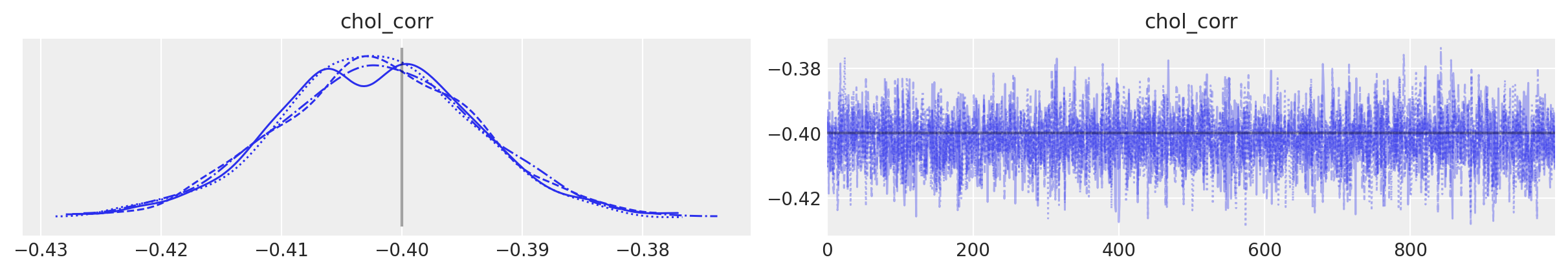
您还可以看到,采样器恢复了真实的均值、相关性和标准差。通常,在图表中会更清晰
az.plot_trace(
    trace,
    var_names="chol_corr",
    coords={"axis": "y", "axis_bis": "z"},
    lines=[("chol_corr", {}, Rho_actual[0, 1])],
);
az.plot_trace(
    trace,
    var_names=["~chol", "~chol_corr"],
    compact=True,
    lines=[
        ("mu", {}, mu_actual),
        ("cov", {}, Sigma_actual),
        ("chol_stds", {}, sigmas_actual),
    ],
);
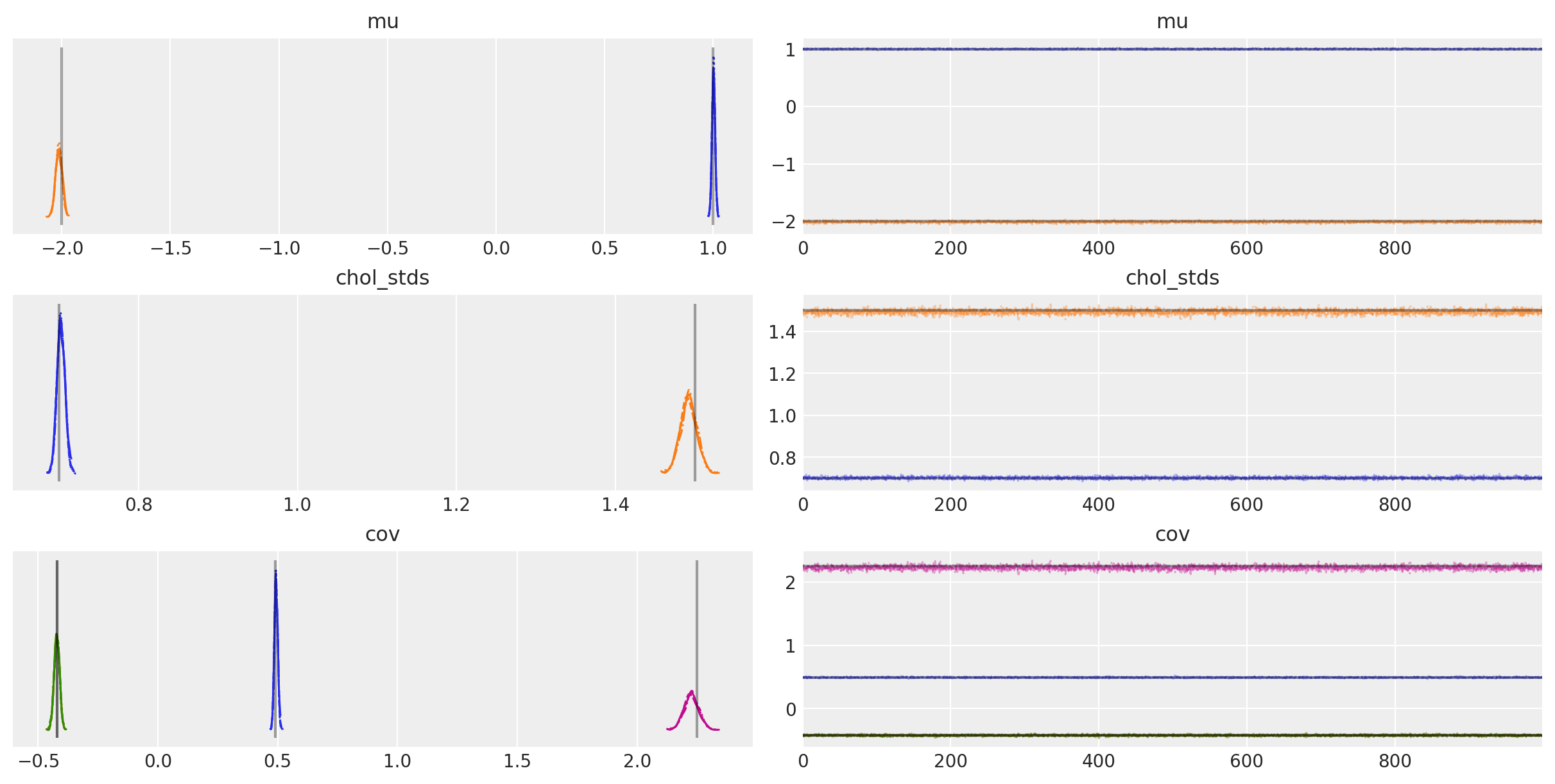
后验期望值非常接近每个分量的真实值!到底有多接近?让我们计算 \(\mu\) 和 \(\Sigma\) 的接近百分比
mu_post = trace.posterior["mu"].mean(("chain", "draw")).values
(1 - mu_post / mu_actual).round(2)
array([-0. , -0.01])
Sigma_post = trace.posterior["cov"].mean(("chain", "draw")).values
(1 - Sigma_post / Sigma_actual).round(2)
array([[-0.01, -0.  ],
       [-0.  ,  0.01]])
因此,后验均值在 \(\mu\) 和 \(\Sigma\) 真实值的 1% 以内。
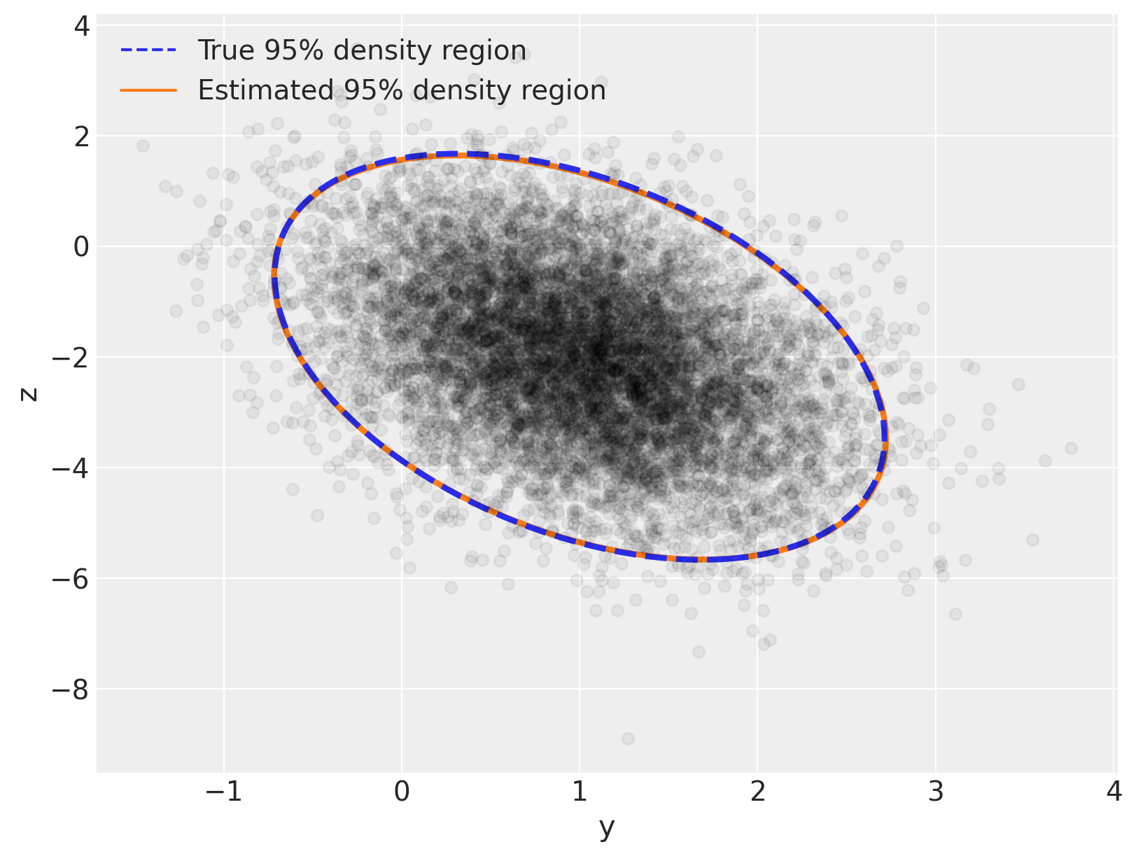
现在让我们复制我们在开头所做的图,但让我们将后验分布叠加在真实分布之上 - 您将看到两者之间具有极佳的视觉一致性
var_post, U_post = np.linalg.eig(Sigma_post)
angle_post = 180.0 / np.pi * np.arccos(np.abs(U_post[0, 0]))

fig, ax = plt.subplots(figsize=(8, 6))

e = Ellipse(
    mu_actual,
    2 * np.sqrt(5.991 * var[0]),
    2 * np.sqrt(5.991 * var[1]),
    angle=angle,
    linewidth=3,
    linestyle="dashed",
)
e.set_edgecolor("C0")
e.set_zorder(11)
e.set_fill(False)
ax.add_artist(e)

e_post = Ellipse(
    mu_post,
    2 * np.sqrt(5.991 * var_post[0]),
    2 * np.sqrt(5.991 * var_post[1]),
    angle=angle_post,
    linewidth=3,
)
e_post.set_edgecolor("C1")
e_post.set_zorder(10)
e_post.set_fill(False)
ax.add_artist(e_post)

ax.scatter(x[:, 0], x[:, 1], c="k", alpha=0.05, zorder=11)
ax.set_xlabel("y")
ax.set_ylabel("z")

line = Line2D([], [], color="C0", linestyle="dashed", label="True 95% density region")
line_post = Line2D([], [], color="C1", label="Estimated 95% density region")
ax.legend(
    handles=[line, line_post],
    loc=2,
);
%load_ext watermark
%watermark -n -u -v -iv -w -p pytensor,xarray
Last updated: Thu Oct 12 2023

Python implementation: CPython
Python version       : 3.11.6
IPython version      : 8.16.1

pytensor: 2.17.1
xarray  : 2023.9.0

numpy     : 1.25.2
matplotlib: 3.8.0
pymc      : 5.9.0
arviz     : 0.16.1

Watermark: 2.4.3