


如何在 PyMC 中包装 JAX 函数#
import arviz as az
import matplotlib.pyplot as plt
import numpy as np
import pymc as pm
import pytensor
import pytensor.tensor as pt

from pytensor.graph import Apply, Op
RANDOM_SEED = 104109109
rng = np.random.default_rng(RANDOM_SEED)
az.style.use("arviz-darkgrid")
注意
本笔记本使用了一些非 PyMC 依赖库,因此需要专门安装才能运行。打开下面的下拉菜单以获取更多指导。
额外依赖库安装说明
为了运行本笔记本(本地或在 binder 上),您不仅需要一个可用的 PyMC 安装以及所有可选依赖项,还需要安装一些额外的依赖库。有关 PyMC 本身安装的建议,请参阅 安装
您可以使用您偏好的包管理器安装这些依赖库,我们以下面的 pip 和 conda 命令为例。
$ pip install jax numpyro
请注意,如果您想(或需要)从笔记本内部而不是命令行安装软件包,您可以通过运行 pip 命令的变体来安装软件包
import sys
!{sys.executable} -m pip install jax numpyro
您不应运行 !pip install,因为它可能会将软件包安装在不同的环境中,即使安装后也无法从 Jupyter 笔记本中使用。
另一种替代方法是使用 conda
$ conda install jax numpyro
当使用 conda 安装科学 Python 包时,我们建议使用 conda forge
import jax
import jax.numpy as jnp
import jax.scipy as jsp
import pymc.sampling_jax

from pytensor.link.jax.dispatch import jax_funcify
/home/ricardo/miniconda3/envs/pymc-examples/lib/python3.10/site-packages/pytensor/link/jax/dispatch.py:87: UserWarning: JAX omnistaging couldn't be disabled: Disabling of omnistaging is no longer supported in JAX version 0.2.12 and higher: see https://github.com/google/jax/blob/main/design_notes/omnistaging.md.
  warnings.warn(f"JAX omnistaging couldn't be disabled: {e}")
/home/ricardo/Documents/Projects/pymc/pymc/sampling_jax.py:36: UserWarning: This module is experimental.
  warnings.warn("This module is experimental.")
简介:PyTensor 及其后端#
PyMC 使用 PyTensor 库来创建和操作概率图。PyTensor 是后端无关的,这意味着它可以利用用不同语言或框架编写的函数,包括纯 Python、NumPy、C、Cython、Numba 和 JAX。
所有需要做的是将此类函数封装在 PyTensor Op 中,它强制执行关于如何处理纯“操作”的输入和输出的特定 API。它还实现了可选的额外功能的方法,如符号形状推断和自动微分。这在 PyTensor Op 文档 和我们的 使用“黑盒”似然函数 pymc-example 中有详细介绍。
最近,PyTensor 变得能够直接编译到其中一些语言/框架,这意味着我们可以将完整的 PyTensor 图转换为 JAX 或 NUMBA jitted 函数,而传统上它们只能转换为 Python 或 C。
这有一些有趣的用途,例如使用纯 JAX 采样器对 PyMC 中定义的模型进行采样,例如在 NumPyro 或 BlackJax 中实现的那些。
本笔记本演示了我们如何实现一个新的 PyTensor Op 来包装 JAX 函数。
大纲#
我们从与 使用“黑盒”似然函数 中采取的类似路径开始,它将 NumPy 函数包装在 PyTensor
Op中,这次改为包装 JAX jitted 函数。然后,我们使 PyTensor 能够“解包”刚刚包装的 JAX 函数,以便可以将整个图编译为 JAX。我们利用这一点,通过 JAX NumPyro NUTS 采样器对我们的 PyMC 模型进行采样。
一个动机示例:边缘 HMM#
为了说明目的,我们将模拟遵循简单 隐马尔可夫模型 (HMM) 的数据,其中有 3 个可能的潜在状态 \(S \in \{0, 1, 2\}\) 和正态发射似然。
我们的 HMM 将具有固定的类别概率 \(P\) 用于跨状态切换,这仅取决于上一个状态
为了完成我们的模型,我们假设每个可能的初始状态 \(S_{t0}\) 都有固定的概率 \(P_{t0}\),
模拟数据#
让我们根据这个模型生成数据!第一步是为模型中的参数设置一些值
# Emission signal and noise parameters
emission_signal_true = 1.15
emission_noise_true = 0.15

p_initial_state_true = np.array([0.9, 0.09, 0.01])

# Probability of switching from state_t to state_t+1
p_transition_true = np.array(
    [
        #    0,   1,   2
        [0.9, 0.09, 0.01],  # 0
        [0.1, 0.8, 0.1],  # 1
        [0.2, 0.1, 0.7],  # 2
    ]
)

# Confirm that we have defined valid probabilities
assert np.isclose(np.sum(p_initial_state_true), 1)
assert np.allclose(np.sum(p_transition_true, axis=-1), 1)
# Let's compute the log of the probalitiy transition matrix for later use
with np.errstate(divide="ignore"):
    logp_initial_state_true = np.log(p_initial_state_true)
    logp_transition_true = np.log(p_transition_true)

logp_initial_state_true, logp_transition_true
(array([-0.10536052, -2.40794561, -4.60517019]),
 array([[-0.10536052, -2.40794561, -4.60517019],
        [-2.30258509, -0.22314355, -2.30258509],
        [-1.60943791, -2.30258509, -0.35667494]]))
# We will observe 70 HMM processes, each with a total of 50 steps
n_obs = 70
n_steps = 50
我们编写一个辅助函数来生成单个 HMM 过程并创建我们的模拟数据
def simulate_hmm(p_initial_state, p_transition, emission_signal, emission_noise, n_steps, rng):
    """Generate hidden state and emission from our HMM model."""

    possible_states = np.array([0, 1, 2])

    hidden_states = []
    initial_state = rng.choice(possible_states, p=p_initial_state)
    hidden_states.append(initial_state)
    for step in range(n_steps):
        new_hidden_state = rng.choice(possible_states, p=p_transition[hidden_states[-1]])
        hidden_states.append(new_hidden_state)
    hidden_states = np.array(hidden_states)

    emissions = rng.normal(
        (hidden_states + 1) * emission_signal,
        emission_noise,
    )

    return hidden_states, emissions
single_hmm_hidden_state, single_hmm_emission = simulate_hmm(
    p_initial_state_true,
    p_transition_true,
    emission_signal_true,
    emission_noise_true,
    n_steps,
    rng,
)
print(single_hmm_hidden_state)
print(np.round(single_hmm_emission, 2))
[0 0 0 0 0 0 1 1 1 1 1 1 0 0 0 0 0 1 1 1 1 1 1 1 1 1 1 1 1 1 1 1 1 1 2 2 1
 1 1 0 0 0 0 0 0 0 0 0 0 0 0]
[1.34 0.79 1.07 1.25 1.33 0.98 1.97 2.45 2.21 2.19 2.21 2.15 1.24 1.16
 0.78 1.18 1.34 2.21 2.44 2.14 2.15 2.38 2.27 2.33 2.26 2.37 2.45 2.36
 2.35 2.32 2.36 2.21 2.27 2.32 3.68 3.32 2.39 2.14 1.99 1.32 1.15 1.31
 1.25 1.17 1.06 0.91 0.88 1.17 1.   1.01 0.87]
hidden_state_true = []
emission_observed = []

for i in range(n_obs):
    hidden_state, emission = simulate_hmm(
        p_initial_state_true,
        p_transition_true,
        emission_signal_true,
        emission_noise_true,
        n_steps,
        rng,
    )
    hidden_state_true.append(hidden_state)
    emission_observed.append(emission)

hidden_state = np.array(hidden_state_true)
emission_observed = np.array(emission_observed)
fig, ax = plt.subplots(2, 1, figsize=(8, 6), sharex=True)
# Plot first five hmm processes
for i in range(4):
    ax[0].plot(hidden_state_true[i] + i * 0.02, color=f"C{i}", lw=2, alpha=0.4)
    ax[1].plot(emission_observed[i], color=f"C{i}", lw=2, alpha=0.4)
ax[0].set_yticks([0, 1, 2])
ax[0].set_ylabel("hidden state")
ax[1].set_ylabel("observed emmission")
ax[1].set_xlabel("step")
fig.suptitle("Simulated data");
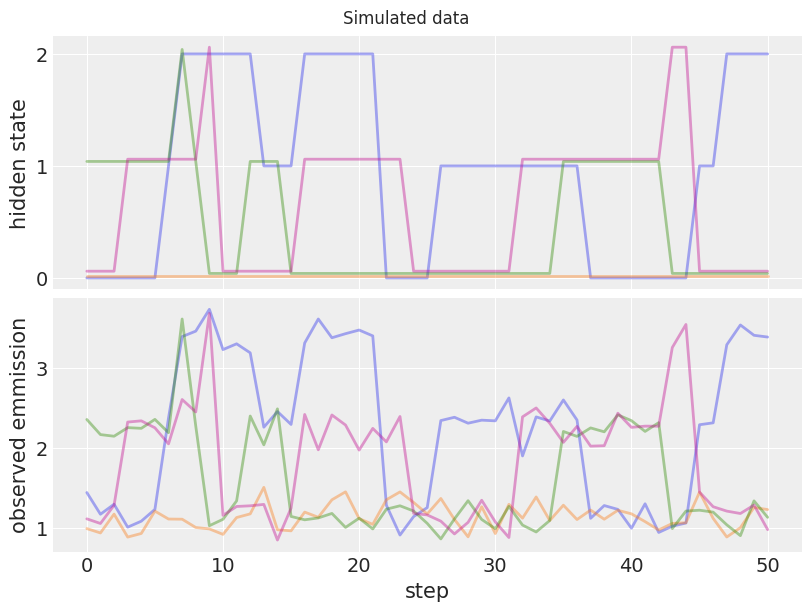
上图显示了隐藏状态和我们模拟数据的相应观测发射。稍后,我们将使用这些数据对真实模型参数执行后验推断。
使用 JAX 计算边缘 HMM 似然#
我们将编写一个 JAX 函数来计算我们的 HMM 模型的似然,对隐藏状态进行边缘化处理。这可以更有效地对剩余的模型参数进行采样。为了实现这一点,我们将使用众所周知的 前向算法,在对数尺度上工作以获得数值稳定性。
我们将利用 JAX scan 来获得高效且可微分的对数似然,并使用方便的 vmap 在多个观测过程之间自动向量化此对数似然。
我们的核心 JAX 函数计算单个 HMM 过程的边缘对数似然
def hmm_logp(
    emission_observed,
    emission_signal,
    emission_noise,
    logp_initial_state,
    logp_transition,
):
    """Compute the marginal log-likelihood of a single HMM process."""

    hidden_states = np.array([0, 1, 2])

    # Compute log-likelihood of observed emissions for each (step x possible hidden state)
    logp_emission = jsp.stats.norm.logpdf(
        emission_observed[:, None],
        (hidden_states + 1) * emission_signal,
        emission_noise,
    )

    # We use the forward_algorithm to compute log_alpha(x_t) = logp(x_t, y_1:t)
    log_alpha = logp_initial_state + logp_emission[0]
    log_alpha, _ = jax.lax.scan(
        f=lambda log_alpha_prev, logp_emission: (
            jsp.special.logsumexp(log_alpha_prev + logp_transition.T, axis=-1) + logp_emission,
            None,
        ),
        init=log_alpha,
        xs=logp_emission[1:],
    )

    return jsp.special.logsumexp(log_alpha)
Let’s test it with the true parameters and the first simulated HMM process
hmm_logp(
    emission_observed[0],
    emission_signal_true,
    emission_noise_true,
    logp_initial_state_true,
    logp_transition_true,
)
WARNING:absl:No GPU/TPU found, falling back to CPU. (Set TF_CPP_MIN_LOG_LEVEL=0 and rerun for more info.)
DeviceArray(-3.93533794, dtype=float64)
We now use vmap to vectorize the core function across multiple observations.
def vec_hmm_logp(*args):
    vmap = jax.vmap(
        hmm_logp,
        # Only the first argument, needs to be vectorized
        in_axes=(0, None, None, None, None),
    )
    # For simplicity we sum across all the HMM processes
    return jnp.sum(vmap(*args))


# We jit it for better performance!
jitted_vec_hmm_logp = jax.jit(vec_hmm_logp)
Passing a row matrix with only the first simulated HMM process should return the same result
jitted_vec_hmm_logp(
    emission_observed[0][None, :],
    emission_signal_true,
    emission_noise_true,
    logp_initial_state_true,
    logp_transition_true,
)
DeviceArray(-3.93533794, dtype=float64)
Our goal is, however, to compute the joint log-likelihood for all the simulated data
jitted_vec_hmm_logp(
    emission_observed,
    emission_signal_true,
    emission_noise_true,
    logp_initial_state_true,
    logp_transition_true,
)
DeviceArray(-37.00348857, dtype=float64)
We will also ask JAX to give us the function of the gradients with respect to each input. This will come in handy later.
jitted_vec_hmm_logp_grad = jax.jit(jax.grad(vec_hmm_logp, argnums=list(range(5))))
Let’s print out the gradient with respect to emission_signal. We will check this value is unchanged after we wrap our function in PyTensor.
jitted_vec_hmm_logp_grad(
    emission_observed,
    emission_signal_true,
    emission_noise_true,
    logp_initial_state_true,
    logp_transition_true,
)[1]
DeviceArray(-297.86490611, dtype=float64, weak_type=True)
在 PyTensor 中包装 JAX 函数#
现在我们准备将我们的 JAX jitted 函数包装在 PyTensor Op 中,然后我们可以在我们的 PyMC 模型中使用它。 如果您想更详细地了解它,我们建议您查看 PyTensor 的官方 Op 文档。
In brief, we will inherit from Op and define the following methods
make_node: Creates anApplynode that holds together the symbolic inputs and outputs of our operationperform: Python code that returns the evaluation of our operation, given concrete input valuesgrad: Returns a PyTensor symbolic graph that represents the gradient expression of an output cost wrt to its inputs
For the grad we will create a second Op that wraps our jitted grad version from above
class HMMLogpOp(Op):
    def make_node(
        self,
        emission_observed,
        emission_signal,
        emission_noise,
        logp_initial_state,
        logp_transition,
    ):
        # Convert our inputs to symbolic variables
        inputs = [
            pt.as_tensor_variable(emission_observed),
            pt.as_tensor_variable(emission_signal),
            pt.as_tensor_variable(emission_noise),
            pt.as_tensor_variable(logp_initial_state),
            pt.as_tensor_variable(logp_transition),
        ]
        # Define the type of the output returned by the wrapped JAX function
        outputs = [pt.dscalar()]
        return Apply(self, inputs, outputs)

    def perform(self, node, inputs, outputs):
        result = jitted_vec_hmm_logp(*inputs)
        # PyTensor raises an error if the dtype of the returned output is not
        # exactly the one expected from the Apply node (in this case
        # `dscalar`, which stands for float64 scalar), so we make sure
        # to convert to the expected dtype. To avoid unnecessary conversions
        # you should make sure the expected output defined in `make_node`
        # is already of the correct dtype
        outputs[0][0] = np.asarray(result, dtype=node.outputs[0].dtype)

    def grad(self, inputs, output_gradients):
        (
            grad_wrt_emission_obsered,
            grad_wrt_emission_signal,
            grad_wrt_emission_noise,
            grad_wrt_logp_initial_state,
            grad_wrt_logp_transition,
        ) = hmm_logp_grad_op(*inputs)
        # If there are inputs for which the gradients will never be needed or cannot
        # be computed, `pytensor.gradient.grad_not_implemented` should  be used as the
        # output gradient for that input.
        output_gradient = output_gradients[0]
        return [
            output_gradient * grad_wrt_emission_obsered,
            output_gradient * grad_wrt_emission_signal,
            output_gradient * grad_wrt_emission_noise,
            output_gradient * grad_wrt_logp_initial_state,
            output_gradient * grad_wrt_logp_transition,
        ]


class HMMLogpGradOp(Op):
    def make_node(
        self,
        emission_observed,
        emission_signal,
        emission_noise,
        logp_initial_state,
        logp_transition,
    ):
        inputs = [
            pt.as_tensor_variable(emission_observed),
            pt.as_tensor_variable(emission_signal),
            pt.as_tensor_variable(emission_noise),
            pt.as_tensor_variable(logp_initial_state),
            pt.as_tensor_variable(logp_transition),
        ]
        # This `Op` will return one gradient per input. For simplicity, we assume
        # each output is of the same type as the input. In practice, you should use
        # the exact dtype to avoid overhead when saving the results of the computation
        # in `perform`
        outputs = [inp.type() for inp in inputs]
        return Apply(self, inputs, outputs)

    def perform(self, node, inputs, outputs):
        (
            grad_wrt_emission_obsered_result,
            grad_wrt_emission_signal_result,
            grad_wrt_emission_noise_result,
            grad_wrt_logp_initial_state_result,
            grad_wrt_logp_transition_result,
        ) = jitted_vec_hmm_logp_grad(*inputs)
        outputs[0][0] = np.asarray(grad_wrt_emission_obsered_result, dtype=node.outputs[0].dtype)
        outputs[1][0] = np.asarray(grad_wrt_emission_signal_result, dtype=node.outputs[1].dtype)
        outputs[2][0] = np.asarray(grad_wrt_emission_noise_result, dtype=node.outputs[2].dtype)
        outputs[3][0] = np.asarray(grad_wrt_logp_initial_state_result, dtype=node.outputs[3].dtype)
        outputs[4][0] = np.asarray(grad_wrt_logp_transition_result, dtype=node.outputs[4].dtype)


# Initialize our `Op`s
hmm_logp_op = HMMLogpOp()
hmm_logp_grad_op = HMMLogpGradOp()
我们建议使用调试助手 eval 方法来确认我们正确指定了一切。 我们应该得到与之前相同的输出
hmm_logp_op(
    emission_observed,
    emission_signal_true,
    emission_noise_true,
    logp_initial_state_true,
    logp_transition_true,
).eval()
array(-37.00348857)
hmm_logp_grad_op(
    emission_observed,
    emission_signal_true,
    emission_noise_true,
    logp_initial_state_true,
    logp_transition_true,
)[1].eval()
array(-297.86490611)
检查我们的 Op 的梯度是否可以通过 PyTensor grad 接口请求也是有用的
# We define the symbolic `emission_signal` variable outside of the `Op`
# so that we can request the gradient wrt to it
emission_signal_variable = pt.as_tensor_variable(emission_signal_true)
x = hmm_logp_op(
    emission_observed,
    emission_signal_variable,
    emission_noise_true,
    logp_initial_state_true,
    logp_transition_true,
)
x_grad_wrt_emission_signal = pt.grad(x, wrt=emission_signal_variable)
x_grad_wrt_emission_signal.eval()
array(-297.86490611)
使用 PyMC 采样#
现在我们准备使用 PyMC 对我们的 HMM 模型进行推断。 我们将为每个模型参数定义先验,并使用 Potential 将联合对数似然项添加到我们的模型中。
with pm.Model() as model:
    emission_signal = pm.Normal("emission_signal", 0, 1)
    emission_noise = pm.HalfNormal("emission_noise", 1)

    p_initial_state = pm.Dirichlet("p_initial_state", np.ones(3))
    logp_initial_state = pt.log(p_initial_state)

    p_transition = pm.Dirichlet("p_transition", np.ones(3), size=3)
    logp_transition = pt.log(p_transition)

    loglike = pm.Potential(
        "hmm_loglike",
        hmm_logp_op(
            emission_observed,
            emission_signal,
            emission_noise,
            logp_initial_state,
            logp_transition,
        ),
    )
pm.model_to_graphviz(model)

在开始采样之前,我们检查模型初始点处每个变量的 logp。 错误往往以初始概率的 nan 或 -inf 形式表现出来。
initial_point = model.initial_point()
initial_point
{'emission_signal': array(0.),
 'emission_noise_log__': array(0.),
 'p_initial_state_simplex__': array([0., 0.]),
 'p_transition_simplex__': array([[0., 0.],
        [0., 0.],
        [0., 0.]])}
model.point_logps(initial_point)
{'emission_signal': -0.92,
 'emission_noise': -0.73,
 'p_initial_state': -1.5,
 'p_transition': -4.51,
 'hmm_loglike': -9812.67}
我们现在准备好采样了!
with model:
    idata = pm.sample(chains=2, cores=1)
Auto-assigning NUTS sampler...
INFO:pymc:Auto-assigning NUTS sampler...
Initializing NUTS using jitter+adapt_diag...
INFO:pymc:Initializing NUTS using jitter+adapt_diag...
/home/ricardo/Documents/Projects/pymc/pymc/pytensorf.py:1005: UserWarning: The parameter 'updates' of pytensor.function() expects an OrderedDict, got <class 'dict'>. Using a standard dictionary here results in non-deterministic behavior. You should use an OrderedDict if you are using Python 2.7 (collections.OrderedDict for older python), or use a list of (shared, update) pairs. Do not just convert your dictionary to this type before the call as the conversion will still be non-deterministic.
  pytensor_function = pytensor.function(
Sequential sampling (2 chains in 1 job)
INFO:pymc:Sequential sampling (2 chains in 1 job)
NUTS: [emission_signal, emission_noise, p_initial_state, p_transition]
INFO:pymc:NUTS: [emission_signal, emission_noise, p_initial_state, p_transition]
Sampling 2 chains for 1_000 tune and 1_000 draw iterations (2_000 + 2_000 draws total) took 109 seconds.
INFO:pymc:Sampling 2 chains for 1_000 tune and 1_000 draw iterations (2_000 + 2_000 draws total) took 109 seconds.
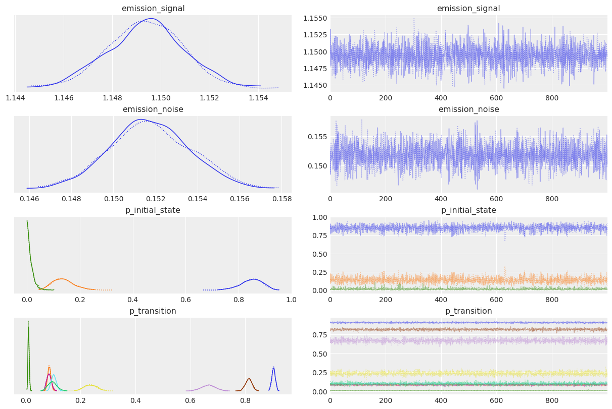
az.plot_trace(idata);
true_values = [
emission_signal_true,
emission_noise_true,
*p_initial_state_true,
*p_transition_true.ravel(),
]
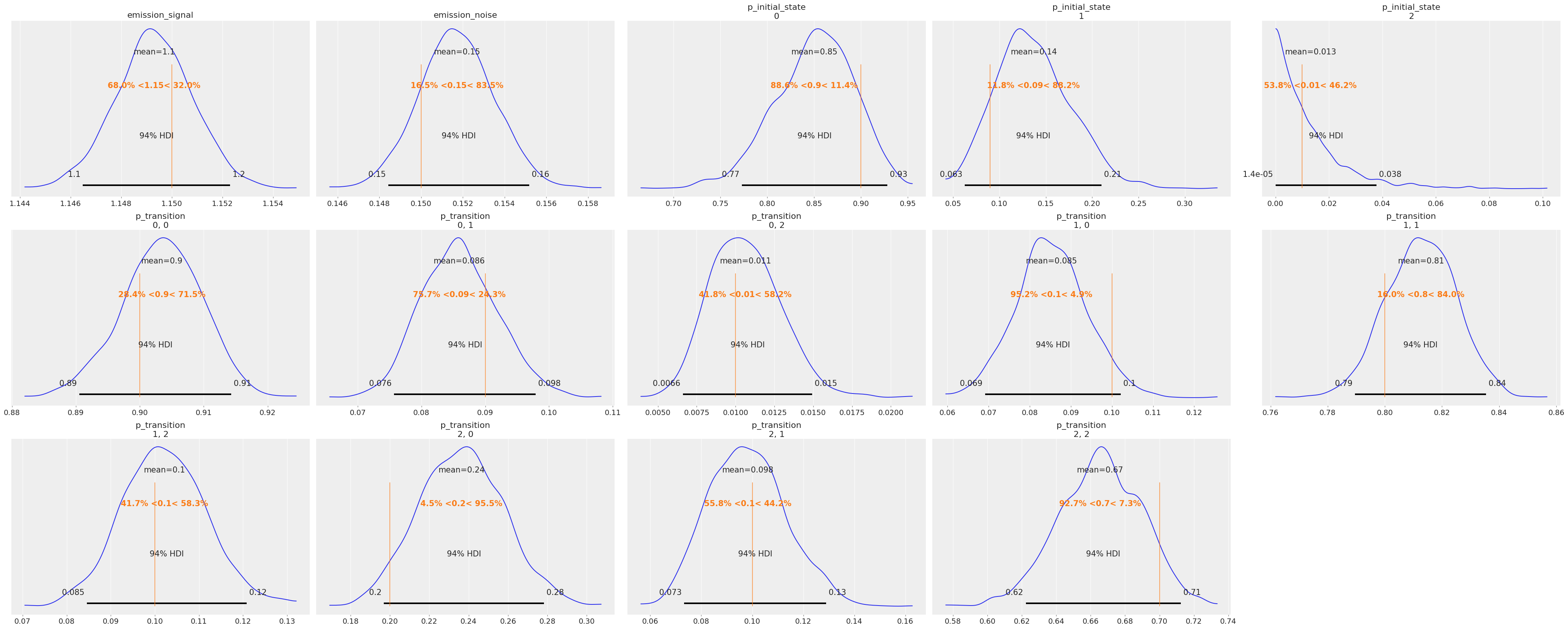
az.plot_posterior(idata, ref_val=true_values, grid=(3, 5));
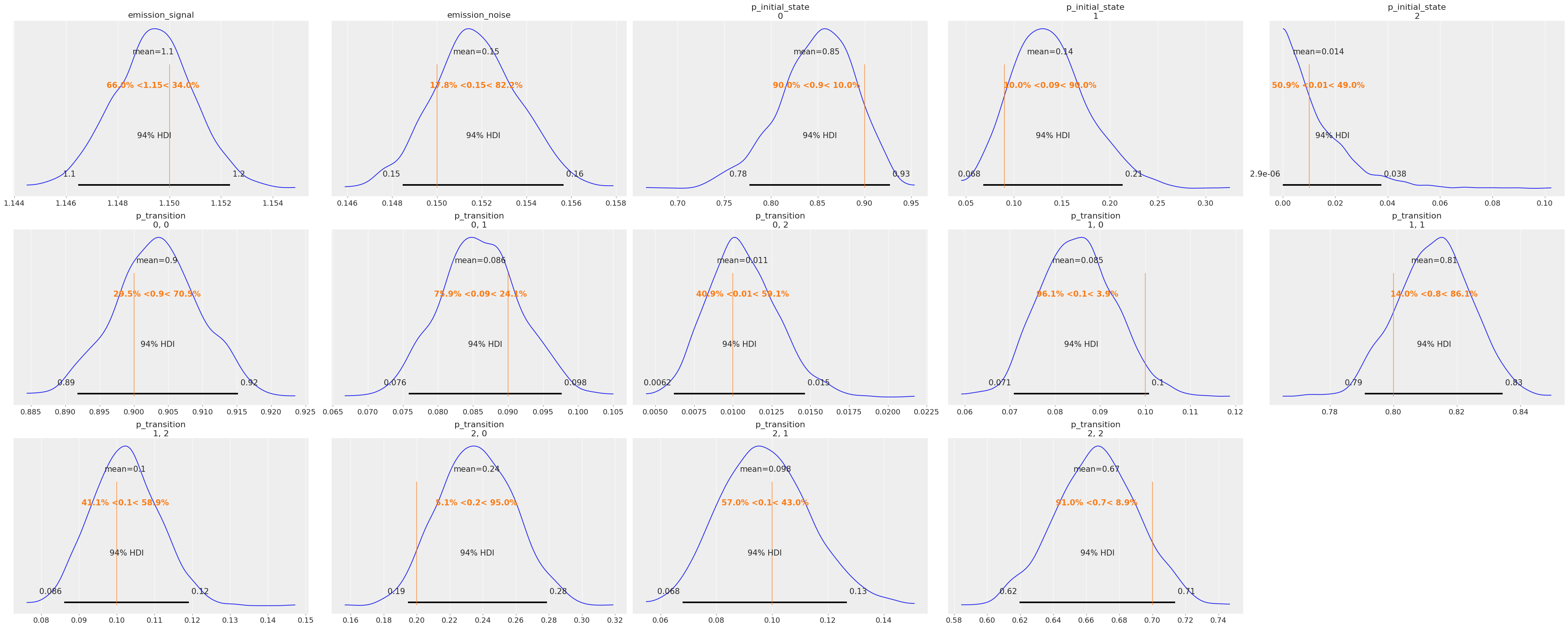
后验分布看起来合理地集中在我们用于生成数据的真实值附近。
解包包装的 JAX 函数#
正如开头提到的,PyTensor 可以将整个图编译为 JAX。 为此,它需要知道图中每个 Op 如何转换为 JAX 函数。 这可以通过 dispatch 和 pytensor.link.jax.dispatch.jax_funcify() 来完成。 大多数默认的 PyTensor Op 已经具有这样的 dispatch 函数,但是我们需要为我们的自定义 HMMLogpOp 添加一个新的,因为 PyTensor 以前从未见过它。
为此,我们需要一个函数,它返回(另一个)JAX 函数,该函数执行与我们的 perform 方法中相同的计算。 幸运的是,我们正是从这样的函数开始的,所以这只需要 3 行简短的代码。
@jax_funcify.register(HMMLogpOp)
def hmm_logp_dispatch(op, **kwargs):
    return vec_hmm_logp
注意
我们不返回 jitted 函数,以便在转换为 JAX 后,整个 PyTensor 图可以一起 jitted。
为了更好地理解 Op JAX 转换,我们建议阅读 PyTensor 的 为 Ops 指南添加 JAX 和 Numba 支持。
我们可以通过使用 mode="JAX" 编译 pytensor.function() 来测试我们的转换函数是否正常工作
out = hmm_logp_op(
    emission_observed,
    emission_signal_true,
    emission_noise_true,
    logp_initial_state_true,
    logp_transition_true,
)
jax_fn = pytensor.function(inputs=[], outputs=out, mode="JAX")
jax_fn()
DeviceArray(-37.00348857, dtype=float64)
我们还可以编译一个 JAX 函数,该函数计算我们 PyMC 模型中每个变量的对数概率,类似于 point_logps()。 我们将使用辅助方法 compile_fn()。
model_logp_jax_fn = model.compile_fn(model.logp(sum=False), mode="JAX")
model_logp_jax_fn(initial_point)
[DeviceArray(-0.91893853, dtype=float64),
 DeviceArray(-0.72579135, dtype=float64),
 DeviceArray(-1.5040774, dtype=float64),
 DeviceArray([-1.5040774, -1.5040774, -1.5040774], dtype=float64),
 DeviceArray(-9812.66649064, dtype=float64)]
请注意,我们可以添加一个同样简单的函数来转换我们的 HMMLogpGradOp,以防我们想要将 PyTensor 梯度图转换为 JAX。 在我们的例子中,我们不需要这样做,因为我们将依靠 JAX grad 函数(或更准确地说,NumPyro 将依靠它)从我们编译的 JAX 函数中再次获得这些。
我们在本文档末尾包含了一个 简短讨论,以帮助您更好地理解使用 PyTensor 图与 JAX 函数之间的权衡,以及您可能希望何时使用其中一种。
使用 NumPyro 采样#
既然我们知道我们的模型 logp 可以完全编译为 JAX,我们可以使用方便的 pymc.sampling_jax.sample_numpyro_nuts() 来使用 NumPyro 中实现的纯 JAX 采样器对我们的模型进行采样。
with model:
    idata_numpyro = pm.sampling_jax.sample_numpyro_nuts(chains=2, progressbar=False)
/home/ricardo/miniconda3/envs/pymc-examples/lib/python3.10/site-packages/tqdm/auto.py:22: TqdmWarning: IProgress not found. Please update jupyter and ipywidgets. See https://ipywidgets.readthedocs.io/en/stable/user_install.html
  from .autonotebook import tqdm as notebook_tqdm
/home/ricardo/Documents/Projects/pymc/pymc/pytensorf.py:1005: UserWarning: The parameter 'updates' of pytensor.function() expects an OrderedDict, got <class 'dict'>. Using a standard dictionary here results in non-deterministic behavior. You should use an OrderedDict if you are using Python 2.7 (collections.OrderedDict for older python), or use a list of (shared, update) pairs. Do not just convert your dictionary to this type before the call as the conversion will still be non-deterministic.
  pytensor_function = pytensor.function(
Compiling...
Compilation time =  0:00:01.897853
Sampling...
Sampling time =  0:00:47.542330
Transforming variables...
Transformation time =  0:00:00.399051
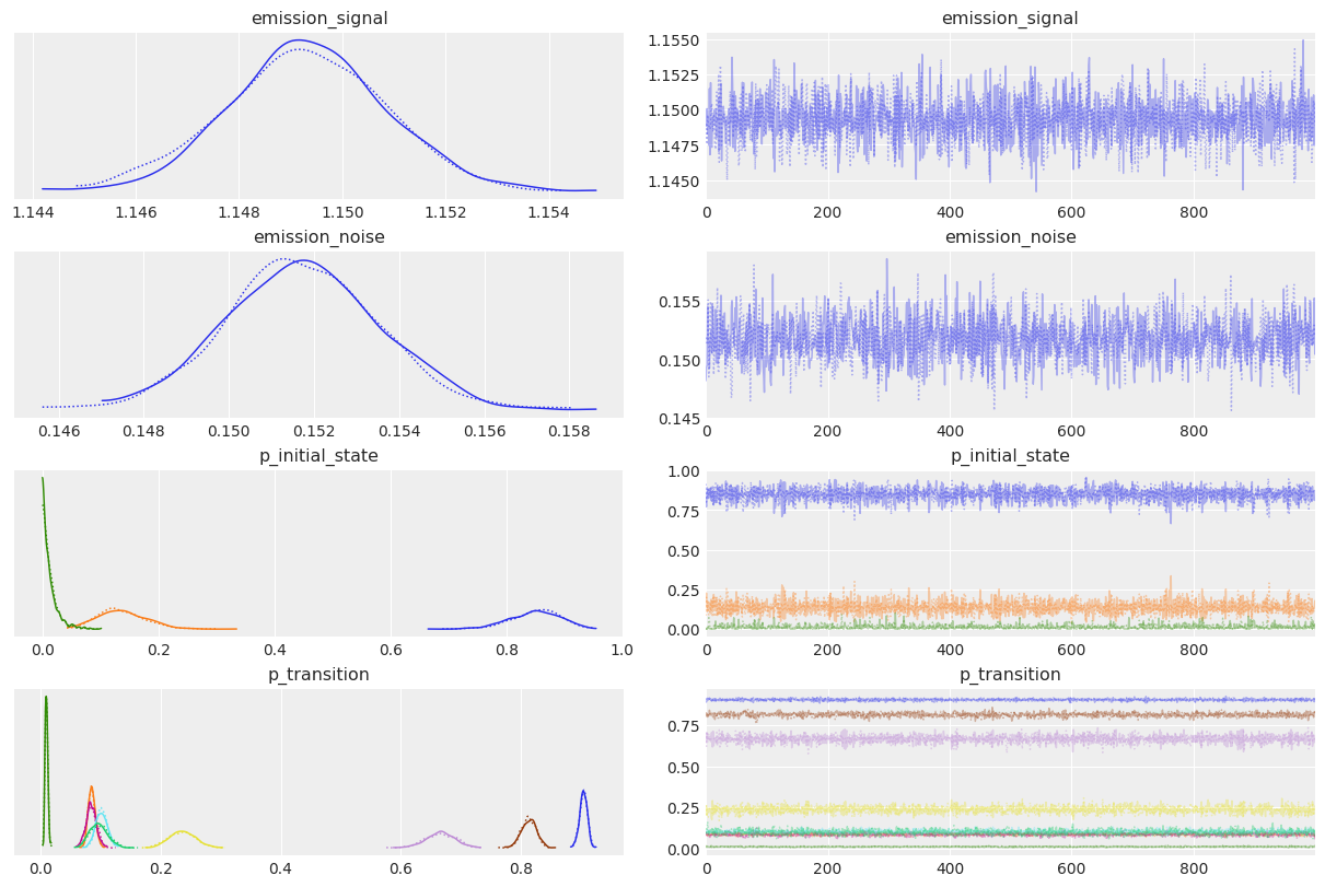
az.plot_trace(idata_numpyro);
az.plot_posterior(idata_numpyro, ref_val=true_values, grid=(3, 5));
正如预期的那样,采样结果看起来非常相似!
根据您使用的模型和计算机架构,纯 JAX 采样器可以提供相当大的加速。
关于使用 PyTensor 与 JAX 的一些简要说明#
何时应该使用 JAX?#
正如我们所见,PyTensor 图和 JAX 函数之间的接口非常简单。
当您想将先前实现的 JAX 函数与 PyMC 模型结合使用时,这非常方便。 在本例中,我们使用了边缘化 HMM 对数似然,但相同的策略可以用于使用深度神经网络或微分方程进行贝叶斯推断,或者几乎任何其他可以在贝叶斯模型上下文中使用的 JAX 实现的函数。
如果您需要利用 JAX 的独特功能,如向量化、对树结构的支持、或其细粒度的并行化以及 GPU 和 TPU 功能,那么它也可能是值得的。
何时不应该使用 JAX?#
与 JAX 一样,PyTensor 的目标是模仿 NumPy 和 Scipy API,以便在 PyTensor 中编写代码应该感觉非常类似于在这些库中编写代码的方式。
然而,使用 PyTensor 也有一些优势
第 2 点意味着如果用 PyTensor 编写,您的图可能会表现更好。 总的来说,您不必担心使用像 log1p 或 logsumexp 这样的专用函数,因为 PyTensor 将能够检测到等效的朴素表达式,并用它们的专用对应物替换它们。 重要的是,当您的图稍后编译为 JAX 时,您仍然可以从这些优化中受益。
问题是 PyTensor 无法推理 JAX 函数,以及包装它们的关联 Op。 这意味着图的“隐藏”在 JAX 函数内部的部分越大,用户从 PyTensor 的重写和调试能力中获益就越少。
第 3 点对于库开发人员来说更为重要。 这是 PyMC 开发人员选择使用 PyTensor(以及之前的其前身 Theano)作为其后端的主要原因。 PyMC 提供的许多面向用户的实用程序都依赖于轻松解析和操作 PyTensor 图的能力。
奖励:使用可以计算自身梯度的单个 Op#
我们必须创建两个 Op,一个用于我们关心的函数,另一个单独用于其梯度。 然而,JAX 提供了一个 value_and_grad 实用程序,它可以同时返回函数的值及其梯度。 如果我们足够聪明,我们可以做类似的事情,并使用单个 Op。
通过这样做,我们可以(可能)节省内存并重用函数及其梯度之间共享的计算。 当处理非常大的 JAX 函数时,这可能很重要。
请注意,如果您有兴趣使用 PyTensor 获取关于您的 Op 的梯度,这才是有用的。 如果您的最终目标是将您的图编译为 JAX,然后再获取梯度(如 NumPyro 所做的那样),那么最好使用第一种方法。 在这种情况下,您甚至不需要实现 grad 方法和关联的 Op。
jitted_hmm_logp_value_and_grad = jax.jit(jax.value_and_grad(vec_hmm_logp, argnums=list(range(5))))
class HmmLogpValueGradOp(Op):
    # By default only show the first output, and "hide" the other ones
    default_output = 0

    def make_node(self, *inputs):
        inputs = [pt.as_tensor_variable(inp) for inp in inputs]
        # We now have one output for the function value, and one output for each gradient
        outputs = [pt.dscalar()] + [inp.type() for inp in inputs]
        return Apply(self, inputs, outputs)

    def perform(self, node, inputs, outputs):
        result, grad_results = jitted_hmm_logp_value_and_grad(*inputs)
        outputs[0][0] = np.asarray(result, dtype=node.outputs[0].dtype)
        for i, grad_result in enumerate(grad_results, start=1):
            outputs[i][0] = np.asarray(grad_result, dtype=node.outputs[i].dtype)

    def grad(self, inputs, output_gradients):
        # The `Op` computes its own gradients, so we call it again.
        value = self(*inputs)
        # We hid the gradient outputs by setting `default_update=0`, but we
        # can retrieve them anytime by accessing the `Apply` node via `value.owner`
        gradients = value.owner.outputs[1:]

        # Make sure the user is not trying to take the gradient with respect to
        # the gradient outputs! That would require computing the second order
        # gradients
        assert all(
            isinstance(g.type, pytensor.gradient.DisconnectedType) for g in output_gradients[1:]
        )

        return [output_gradients[0] * grad for grad in gradients]


hmm_logp_value_grad_op = HmmLogpValueGradOp()
我们再次检查我们可以使用 PyTensor grad 接口获取梯度
emission_signal_variable = pt.as_tensor_variable(emission_signal_true)
# Only the first output is assigned to the variable `x`, due to `default_output=0`
x = hmm_logp_value_grad_op(
    emission_observed,
    emission_signal_variable,
    emission_noise_true,
    logp_initial_state_true,
    logp_transition_true,
)
pt.grad(x, emission_signal_variable).eval()
array(-297.86490611)
水印#
%load_ext watermark
%watermark -n -u -v -iv -w -p pytensor,aeppl,xarray
Last updated: Mon Apr 11 2022

Python implementation: CPython
Python version       : 3.10.2
IPython version      : 8.1.1

pytensor: 2.5.1
aeppl : 0.0.27
xarray: 2022.3.0

matplotlib: 3.5.1
jax       : 0.3.4
pytensor    : 2.5.1
arviz     : 0.12.0
pymc      : 4.0.0b6
numpy     : 1.22.3

Watermark: 2.3.0
许可声明#
本示例库中的所有笔记本均根据 MIT 许可证 提供,该许可证允许修改和重新分发以用于任何用途,前提是保留版权和许可声明。
引用 PyMC 示例#
要引用本笔记本,请使用 Zenodo 为 pymc-examples 存储库提供的 DOI。
重要提示
许多笔记本改编自其他来源:博客、书籍…… 在这种情况下,您也应该引用原始来源。
还请记住引用您的代码使用的相关库。
Here is an citation template in bibtex
@incollection{citekey,
  author    = "<notebook authors, see above>",
  title     = "<notebook title>",
  editor    = "PyMC Team",
  booktitle = "PyMC examples",
  doi       = "10.5281/zenodo.5654871"
}
which once rendered could look like