


Dirichlet 混合多项式#
此示例笔记本演示了如何使用 Dirichlet 混合多项式(也称为 Dirichlet-多项分布 或 DM)来建模分类计数数据。像这样的模型在许多领域都很重要,包括自然语言处理、生态学、生物信息学等等。
Dirichlet-多项分布可以理解为从 多项分布 中抽取的样本,其中每个样本都有略微不同的概率向量,而概率向量本身是从一个共同的 Dirichlet 分布 中抽取的。这与多项分布形成对比,多项分布假设所有观测结果都来自单个固定的概率向量。这使得 Dirichlet-多项分布能够容纳比多项分布更可变的(又名,过度分散的)计数数据。
过度分散的计数分布的其他示例包括 Beta-二项分布 (可以认为是 DM 的一个特例)或 负二项分布。
DM 也是将混合分布在其潜在参数上边缘化的一个示例。本笔记本将演示采用这种方法带来的性能优势。
import arviz as az
import matplotlib.pyplot as plt
import numpy as np
import pymc as pm
import scipy as sp

print(f"Running on PyMC v{pm.__version__}")
Running on PyMC v5.9.0
%config InlineBackend.figure_format = 'retina'
RANDOM_SEED = 8927
rng = np.random.default_rng(RANDOM_SEED)
az.style.use("arviz-darkgrid")
模拟数据#
让我们为此示例模拟一些过度分散的分类计数数据。
在这里,我们正在从 DM 分布本身进行模拟,因此拟合该模型可能有点同义反复,但请放心,像这样的数据确实出现在不同的计数中
文本语料库中的词语 [],
细胞中 RNA 分子的类型 [],
购物者购买的商品 []。
在这里,我们将讨论一个群落生态学示例,假设我们已经观察到 \(k=5\) 种不同树木在 \(n=10\) 个不同森林中的计数。
我们的模拟将生成一个二维整数矩阵(计数),其中每行(从零开始索引)\(i \in (0...n-1)\) 是一个观测值(不同的森林),每列 \(j \in (0...k-1)\) 是一个类别(树种)。我们将使用以下三件事来参数化此分布
\(\mathrm{frac}\) : 每种物种的预期比例,一个 \(k\) 维的单纯形向量(即总和为一)
\(\mathrm{total\_count}\) : 每次观察中统计的项目总数,
\(\mathrm{conc}\) : 浓度,控制我们数据的过度分散,其中较大的值会导致我们的分布更接近多项分布。
在这里,以及在本笔记本中,我们使用了 Dirichlet 分布的 便捷的重参数化,从一个参数到两个参数, \(\alpha=\mathrm{conc} \times \mathrm{frac}\),因为这符合我们期望的解释。
DM 的每次观测都是通过以下方式模拟的
首先获得一个在 \(k\)-单纯形上的值,模拟为 \(p_i \sim \mathrm{Dirichlet}(\alpha=\mathrm{conc} \times \mathrm{frac})\),
然后模拟 \(\mathrm{counts}_i \sim \mathrm{Multinomial}(\mathrm{total\_count}, p_i)\)。
请注意,每次观测都获得其自身的潜在参数 \(p_i\),这些参数是从一个共同的 Dirichlet 分布中独立模拟的。
true_conc = 6.0
true_frac = np.array([0.45, 0.30, 0.15, 0.09, 0.01])
trees = ["pine", "oak", "ebony", "rosewood", "mahogany"]  # Tree species observed
# fmt: off
forests = [  # Forests observed
    "sunderbans", "amazon", "arashiyama", "trossachs", "valdivian",
    "bosc de poblet", "font groga", "monteverde", "primorye", "daintree",
]
# fmt: on
k = len(trees)
n = len(forests)
total_count = 50

true_p = sp.stats.dirichlet(true_conc * true_frac).rvs(size=n, random_state=rng)
observed_counts = np.vstack(
    [sp.stats.multinomial(n=total_count, p=p_i).rvs(random_state=rng) for p_i in true_p]
)

observed_counts
array([[21,  9, 11,  6,  3],
       [36,  7,  6,  1,  0],
       [ 8, 31,  1, 10,  0],
       [25,  4, 17,  4,  0],
       [43,  6,  1,  0,  0],
       [28, 10, 12,  0,  0],
       [21, 16, 10,  3,  0],
       [16, 32,  2,  0,  0],
       [45,  4,  1,  0,  0],
       [35,  5,  2,  8,  0]])
多项式模型#
我们将要拟合到这些数据的第一个模型是普通多项式模型,其中唯一的参数是每个类别的预期比例 \(\mathrm{frac}\),我们将为其提供 Dirichlet 先验。虽然均匀先验(每个 \(j\) 的 \(\alpha_j=1\))效果良好,但如果我们对每种树的比例有独立的信念,我们可以将其编码到我们的先验中,例如,增加我们期望物种-\(j\) 比例更高的 \(\alpha_j\) 的值。
coords = {"tree": trees, "forest": forests}
with pm.Model(coords=coords) as model_multinomial:
    frac = pm.Dirichlet("frac", a=np.ones(k), dims="tree")
    counts = pm.Multinomial(
        "counts", n=total_count, p=frac, observed=observed_counts, dims=("forest", "tree")
    )

pm.model_to_graphviz(model_multinomial)

with model_multinomial:
    trace_multinomial = pm.sample(chains=4)
Auto-assigning NUTS sampler...
Initializing NUTS using jitter+adapt_diag...
Multiprocess sampling (4 chains in 4 jobs)
NUTS: [frac]
Sampling 4 chains for 1_000 tune and 1_000 draw iterations (4_000 + 4_000 draws total) took 2 seconds.
az.plot_trace(data=trace_multinomial, var_names=["frac"]);
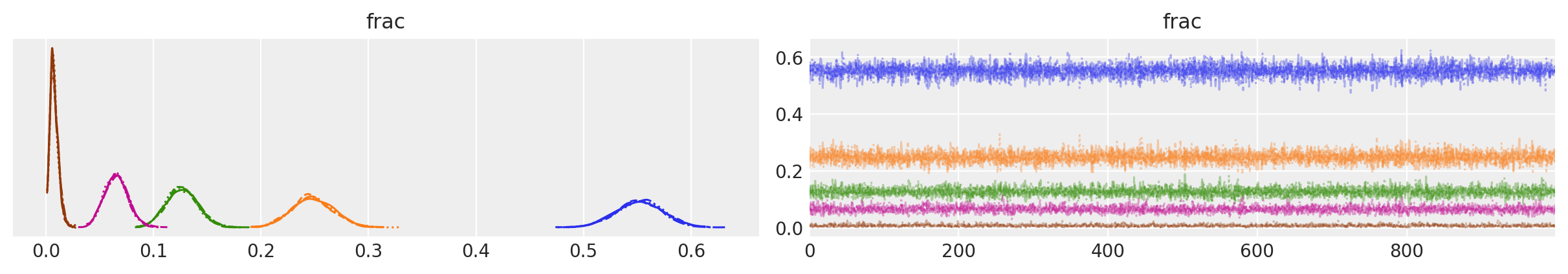
迹图看起来相当不错;从视觉上看,每个参数似乎都在后验分布周围良好地移动。
summary_multinomial = az.summary(trace_multinomial, var_names=["frac"])

summary_multinomial = summary_multinomial.assign(
    ess_bulk_per_sec=lambda x: x.ess_bulk / trace_multinomial.posterior.sampling_time,
)

summary_multinomial
| 均值 | 标准差 | hdi_3% | hdi_97% | mcse_mean | mcse_sd | ess_bulk | ess_tail | r_hat | ess_bulk_per_sec | |
|---|---|---|---|---|---|---|---|---|---|---|
| frac[松树] | 0.552 | 0.022 | 0.510 | 0.591 | 0.0 | 0.0 | 5955.0 | 3480.0 | 1.0 | 2675.351076 |
| frac[橡树] | 0.248 | 0.019 | 0.213 | 0.284 | 0.0 | 0.0 | 5428.0 | 3478.0 | 1.0 | 2438.590368 |
| frac[乌木] | 0.127 | 0.015 | 0.099 | 0.153 | 0.0 | 0.0 | 4773.0 | 3080.0 | 1.0 | 2144.324212 |
| frac[红木] | 0.065 | 0.011 | 0.045 | 0.086 | 0.0 | 0.0 | 3351.0 | 2680.0 | 1.0 | 1505.474636 |
| frac[桃花心木] | 0.008 | 0.004 | 0.001 | 0.015 | 0.0 | 0.0 | 1341.0 | 1277.0 | 1.0 | 602.459411 |
同样,参数汇总表中的诊断结果看起来都不错。在这里,我们添加了一列,用于估计每秒采样的有效样本量。
az.plot_forest(trace_multinomial, var_names=["frac"])
for j, (y_tick, frac_j) in enumerate(zip(plt.gca().get_yticks(), reversed(true_frac))):
    plt.vlines(frac_j, ymin=y_tick - 0.45, ymax=y_tick + 0.45, color="black", linestyle="--")
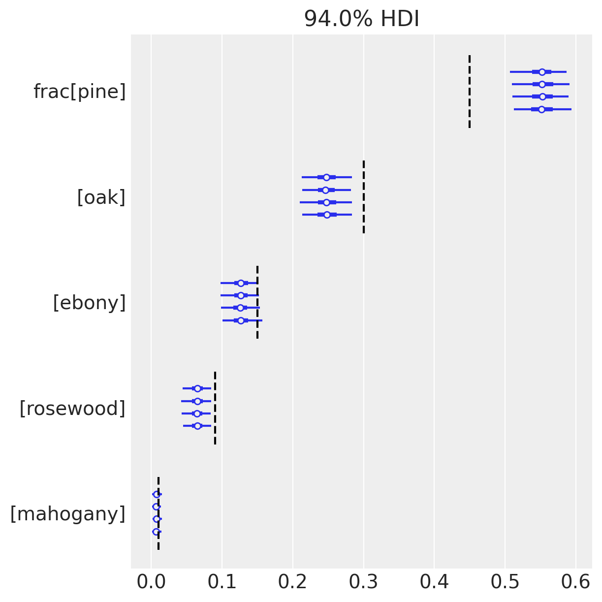
在这里,我们绘制了一个森林图,显示了来自我们的后验近似的均值和 94% HDI。有趣的是,因为我们知道每种物种的潜在频率(虚线),所以我们可以评论我们的推断的准确性。现在,我们模型的问题变得明显了;请注意,94% HDI *不包括* 树种 0、1、3 的真实值。我们可能已经看到 *一个* HDI 遗漏,但是 *三个*???
...怎么回事?
让我们使用后验预测检查来排除此模型的故障,将我们的数据与根据我们的后验估计模拟的数据进行比较。
with model_multinomial:
    pp_samples = pm.sample_posterior_predictive(trace=trace_multinomial)

# Concatenate with InferenceData object
trace_multinomial.extend(pp_samples)
Sampling: [counts]
cmap = plt.get_cmap("tab10")

fig, axs = plt.subplots(k, 1, sharex=True, sharey=True, figsize=(6, 8))
for j, ax in enumerate(axs):
    c = cmap(j)
    ax.hist(
        trace_multinomial.posterior_predictive.counts.sel(tree=trees[j]).values.flatten(),
        bins=np.arange(total_count),
        histtype="step",
        color=c,
        density=True,
        label="Post.Pred.",
    )
    ax.hist(
        (trace_multinomial.observed_data.counts.sel(tree=trees[j]).values.flatten()),
        bins=np.arange(total_count),
        color=c,
        density=True,
        alpha=0.25,
        label="Observed",
    )
    ax.axvline(
        true_frac[j] * total_count,
        color=c,
        lw=1.0,
        alpha=0.45,
        label="True",
    )
    ax.annotate(
        f"{trees[j]}",
        xy=(0.96, 0.9),
        xycoords="axes fraction",
        ha="right",
        va="top",
        color=c,
    )

axs[-1].legend(loc="upper center", fontsize=10)
axs[-1].set_xlabel("Count")
axs[-1].set_yticks([0, 0.5, 1.0])
axs[-1].set_ylim(0, 0.6);
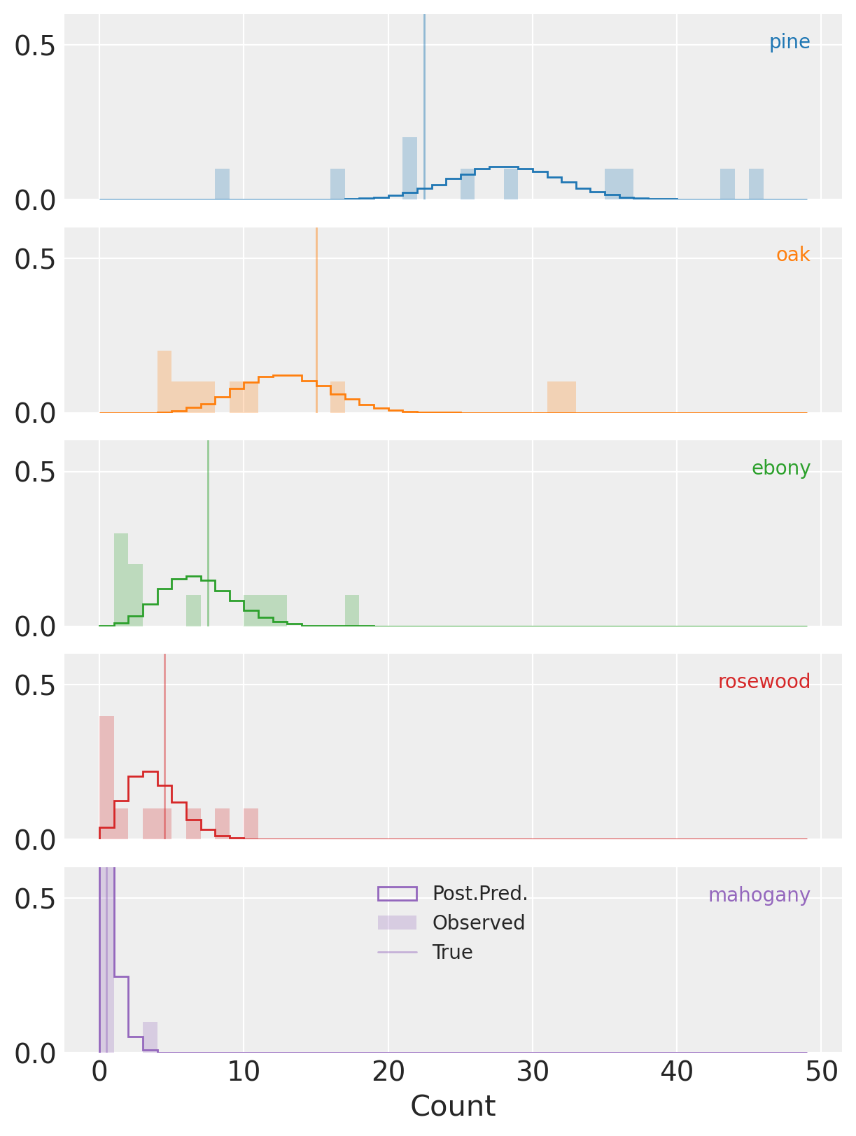
在这里,我们绘制了每个物种的预测计数与观察计数的直方图。
(请注意,y 轴不是完整高度,并且剪切了紫色 桃花心木 物种的分布。)
现在我们可以开始明白为什么我们的后验 HDI 偏离了五种物种中三种的 *真实* 参数(垂直线)。请注意,对于所有物种,观察到的计数通常与以后验分布为条件的预测相差甚远。这对于(例如) 橡树 尤其明显,我们在其中观察到超过 30 棵这种树种,尽管后验预测质量集中在远低于该值的位置。
这就是过度分散的作用,并且清楚地表明我们需要调整我们的模型以适应它。
后验预测检查是诊断模型错误指定的最佳方法之一,本示例也不例外。
Dirichlet-多项式模型 - 显式混合#
让我们继续使用 DM 分布对我们的数据进行建模。
对于此模型,我们将保留对每种物种的预期频率 \(\mathrm{frac}\) 相同的先验。我们还将添加一个严格为正的参数 \(\mathrm{conc}\) 用于浓度。
在我们模型的此迭代中,我们将显式包含潜在多项式概率 \(p_i\),建模来自我们模拟的 \(\mathrm{true\_p}_i\)(我们在现实世界中不会观察到)。
with pm.Model(coords=coords) as model_dm_explicit:
    frac = pm.Dirichlet("frac", a=np.ones(k), dims="tree")
    conc = pm.Lognormal("conc", mu=1, sigma=1)
    p = pm.Dirichlet("p", a=frac * conc, dims=("forest", "tree"))
    counts = pm.Multinomial(
        "counts", n=total_count, p=p, observed=observed_counts, dims=("forest", "tree")
    )

pm.model_to_graphviz(model_dm_explicit)

将此图表与第一个图表进行比较。在这里,潜在的 Dirichlet 分布 \(p\) 将多项式与预期频率 \(\mathrm{frac}\) 分开,从而解释了相对于简单多项式模型的计数过度分散。
with model_dm_explicit:
    trace_dm_explicit = pm.sample(chains=4, target_accept=0.9)
Auto-assigning NUTS sampler...
Initializing NUTS using jitter+adapt_diag...
Multiprocess sampling (4 chains in 4 jobs)
NUTS: [frac, conc, p]
Sampling 4 chains for 1_000 tune and 1_000 draw iterations (4_000 + 4_000 draws total) took 87 seconds.
The rhat statistic is larger than 1.01 for some parameters. This indicates problems during sampling. See https://arxiv.org/abs/1903.08008 for details
The effective sample size per chain is smaller than 100 for some parameters.  A higher number is needed for reliable rhat and ess computation. See https://arxiv.org/abs/1903.08008 for details
There were 16 divergences after tuning. Increase `target_accept` or reparameterize.
在这里,我们必须将 target_accept 从 0.8 增加到 0.9,以免淹没在发散中。
我们还收到了关于 rhat 统计量的警告,尽管我们现在将忽略它。更有趣的是,采样此模型比第一个模型花费的时间要长得多。部分原因是我们的模型具有额外的约 \((n \times k)\) 个参数,但似乎 NUTS 也存在其他几何挑战。
我们将看看是否可以在下一个模型中修复这些问题,但现在让我们看一下迹线。
az.plot_trace(data=trace_dm_explicit, var_names=["frac", "conc"]);
当稀有物种(桃花心木)的估计比例非常接近于零时,似乎会发生发散。
az.plot_forest(trace_dm_explicit, var_names=["frac"])
for j, (y_tick, frac_j) in enumerate(zip(plt.gca().get_yticks(), reversed(true_frac))):
    plt.vlines(frac_j, ymin=y_tick - 0.45, ymax=y_tick + 0.45, color="black", linestyle="--")
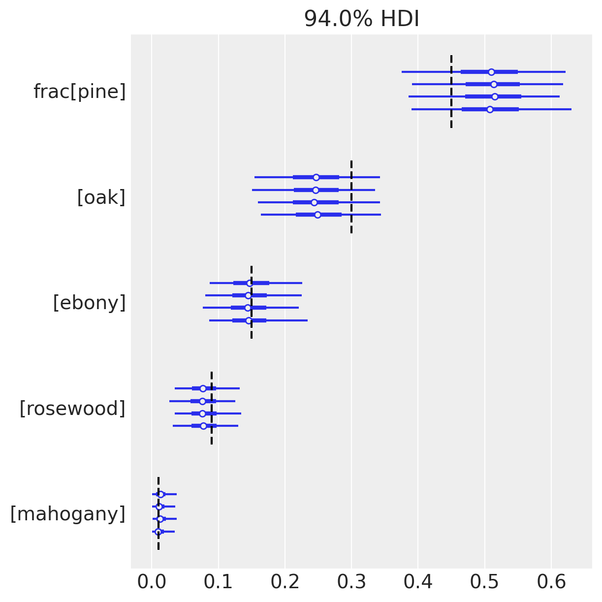
另一方面,由于我们知道 \(\mathrm{frac}\) 的真实值,我们可以祝贺自己,HDI 包括我们所有物种的真实值!
对这种混合物进行建模使我们的推断对计数的过度分散具有鲁棒性,而普通多项式模型非常敏感。请注意,每个 \(\mathrm{frac}_i\) 的 HDI 比以前宽得多。在这种情况下,这使得正确和不正确的推断之间存在差异。
summary_dm_explicit = az.summary(trace_dm_explicit, var_names=["frac", "conc"])
summary_dm_explicit = summary_dm_explicit.assign(
    ess_bulk_per_sec=lambda x: x.ess_bulk / trace_dm_explicit.posterior.sampling_time,
)

summary_dm_explicit
| 均值 | 标准差 | hdi_3% | hdi_97% | mcse_mean | mcse_sd | ess_bulk | ess_tail | r_hat | ess_bulk_per_sec | |
|---|---|---|---|---|---|---|---|---|---|---|
| frac[松树] | 0.509 | 0.063 | 0.386 | 0.622 | 0.001 | 0.001 | 4102.0 | 3040.0 | 1.00 | 47.028042 |
| frac[橡树] | 0.248 | 0.050 | 0.158 | 0.343 | 0.001 | 0.000 | 5036.0 | 2996.0 | 1.00 | 57.736036 |
| frac[乌木] | 0.149 | 0.040 | 0.082 | 0.227 | 0.001 | 0.000 | 3379.0 | 2915.0 | 1.00 | 38.739091 |
| frac[红木] | 0.080 | 0.028 | 0.031 | 0.131 | 0.001 | 0.000 | 2147.0 | 2488.0 | 1.00 | 24.614628 |
| frac[桃花心木] | 0.014 | 0.012 | 0.000 | 0.036 | 0.001 | 0.001 | 69.0 | 109.0 | 1.04 | 0.791062 |
| 浓度 | 5.712 | 1.741 | 2.729 | 8.872 | 0.036 | 0.026 | 2209.0 | 2082.0 | 1.00 | 25.325437 |
这很棒,但是 *我们可以做得更好*。frac[桃花心木] 的略微过大的 \(\hat{R}\) 值有点令人担忧,并且令人惊讶的是我们的 \(\mathrm{ESS} \; \mathrm{sec}^{-1}\) 非常小。
Dirichlet-多项式模型 - 边缘化#
令人高兴的是,Dirichlet 分布与多项式共轭,因此对于边缘化分布,即 Dirichlet-多项式分布,有一个方便的闭式解,该分布已在 3.11.0 中添加到 PyMC。
让我们利用这一点,边缘化显式潜在参数 \(p_i\),用 DM 替换此节点和多项式的组合,以创建一个等效的模型。
with pm.Model(coords=coords) as model_dm_marginalized:
    frac = pm.Dirichlet("frac", a=np.ones(k), dims="tree")
    conc = pm.Lognormal("conc", mu=1, sigma=1)
    counts = pm.DirichletMultinomial(
        "counts", n=total_count, a=frac * conc, observed=observed_counts, dims=("forest", "tree")
    )

pm.model_to_graphviz(model_dm_marginalized)

板块图显示,我们已将曾经是潜在 Dirichlet 节点和多项式节点的节点折叠到单个 DM 节点中。
with model_dm_marginalized:
    trace_dm_marginalized = pm.sample(chains=4)
Auto-assigning NUTS sampler...
Initializing NUTS using jitter+adapt_diag...
Multiprocess sampling (4 chains in 4 jobs)
NUTS: [frac, conc]
Sampling 4 chains for 1_000 tune and 1_000 draw iterations (4_000 + 4_000 draws total) took 2 seconds.
它的采样速度更快,并且没有任何之前的警告!
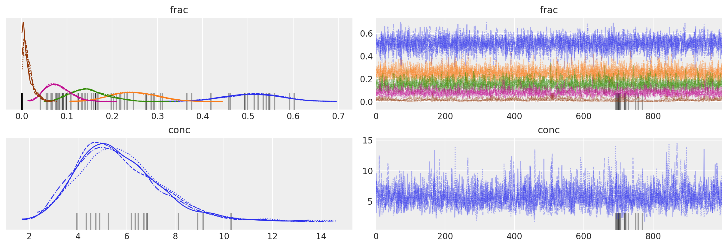
az.plot_trace(data=trace_dm_marginalized, var_names=["frac", "conc"]);

迹图看起来模糊,KDE 很干净。
summary_dm_marginalized = az.summary(trace_dm_marginalized, var_names=["frac", "conc"])
summary_dm_marginalized = summary_dm_marginalized.assign(
    ess_mean_per_sec=lambda x: x.ess_bulk / trace_dm_marginalized.posterior.sampling_time,
)
assert all(summary_dm_marginalized.r_hat < 1.03)

summary_dm_marginalized
| 均值 | 标准差 | hdi_3% | hdi_97% | mcse_mean | mcse_sd | ess_bulk | ess_tail | r_hat | ess_mean_per_sec | |
|---|---|---|---|---|---|---|---|---|---|---|
| frac[松树] | 0.507 | 0.063 | 0.385 | 0.619 | 0.001 | 0.001 | 4330.0 | 2816.0 | 1.0 | 1870.135862 |
| frac[橡树] | 0.248 | 0.051 | 0.150 | 0.341 | 0.001 | 0.000 | 6017.0 | 3571.0 | 1.0 | 2598.754615 |
| frac[乌木] | 0.150 | 0.040 | 0.080 | 0.226 | 0.001 | 0.000 | 4315.0 | 3296.0 | 1.0 | 1863.657331 |
| frac[红木] | 0.079 | 0.028 | 0.031 | 0.130 | 0.000 | 0.000 | 3027.0 | 2718.0 | 1.0 | 1307.367495 |
| frac[桃花心木] | 0.016 | 0.011 | 0.001 | 0.036 | 0.000 | 0.000 | 2856.0 | 2172.0 | 1.0 | 1233.512245 |
| 浓度 | 5.692 | 1.719 | 2.807 | 9.045 | 0.028 | 0.020 | 3594.0 | 2925.0 | 1.0 | 1552.255956 |
我们看到 \(\hat{R}\) 在各处都接近 \(1\),并且 \(\mathrm{ESS} \; \mathrm{sec}^{-1}\) 高得多。我们的重参数化(边缘化)大大提高了采样! (并且,值得庆幸的是,HDI 看起来与其他模型相似。)
这一切看起来都非常好,但是如果我们没有真实值怎么办?
后验预测检查再次拯救了我们!
with model_dm_marginalized:
    pp_samples = pm.sample_posterior_predictive(trace_dm_marginalized)

# Concatenate with InferenceData object
trace_dm_marginalized.extend(pp_samples)
Sampling: [counts]
cmap = plt.get_cmap("tab10")

fig, axs = plt.subplots(k, 2, sharex=True, sharey=True, figsize=(8, 8))
for j, row in enumerate(axs):
    c = cmap(j)
    for _trace, ax in zip([trace_dm_marginalized, trace_multinomial], row):
        ax.hist(
            _trace.posterior_predictive.counts.sel(tree=trees[j]).values.flatten(),
            bins=np.arange(total_count),
            histtype="step",
            color=c,
            density=True,
            label="Post.Pred.",
        )
        ax.hist(
            (_trace.observed_data.counts.sel(tree=trees[j]).values.flatten()),
            bins=np.arange(total_count),
            color=c,
            density=True,
            alpha=0.25,
            label="Observed",
        )
        ax.axvline(
            true_frac[j] * total_count,
            color=c,
            lw=1.0,
            alpha=0.45,
            label="True",
        )
    row[1].annotate(
        f"{trees[j]}",
        xy=(0.96, 0.9),
        xycoords="axes fraction",
        ha="right",
        va="top",
        color=c,
    )

axs[-1, -1].legend(loc="upper center", fontsize=10)
axs[0, 1].set_title("Multinomial")
axs[0, 0].set_title("Dirichlet-multinomial")
axs[-1, 0].set_xlabel("Count")
axs[-1, 1].set_xlabel("Count")
axs[-1, 0].set_yticks([0, 0.5, 1.0])
axs[-1, 0].set_ylim(0, 0.6)
ax.set_ylim(0, 0.6);
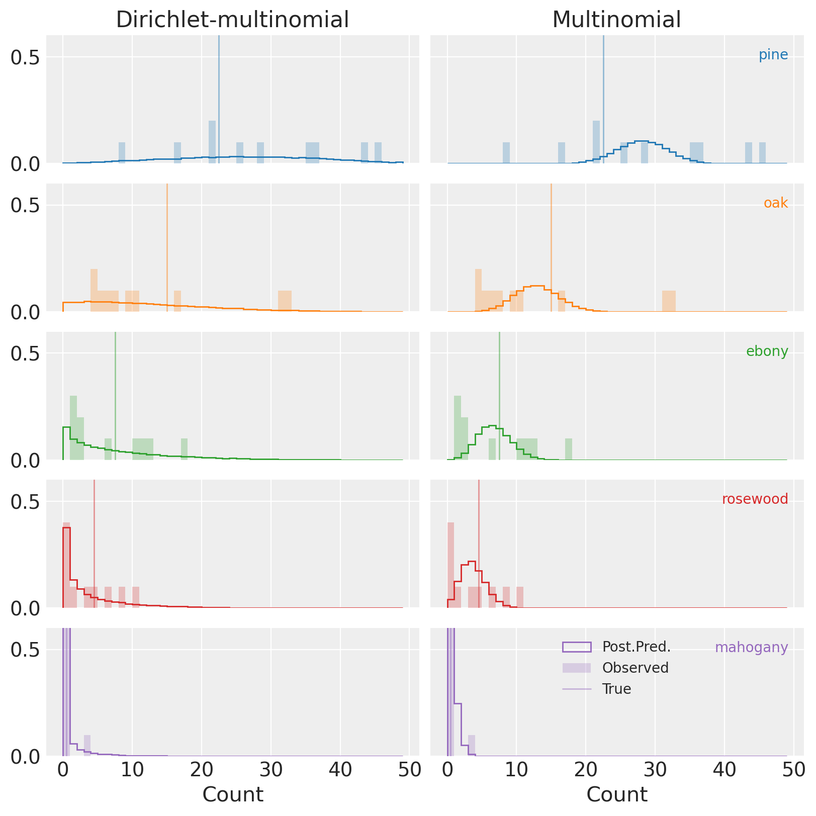
(再次注意,y 轴不是完整高度,并且剪切了紫色 桃花心木 的分布。)
与多项式(右侧的图)相比,DM(左侧)的 PPC 表明,观察到的数据是我们模型完全合理的实现。这是个好消息!
模型比较#
让我们更进一步,尝试量化我们的 DM 模型相对于原始多项式模型的优势程度。我们将使用留一法交叉验证来比较两者的样本外预测能力。
with model_multinomial:
    pm.compute_log_likelihood(trace_multinomial)

with model_dm_marginalized:
    pm.compute_log_likelihood(trace_dm_marginalized)

az.compare(
    {"multinomial": trace_multinomial, "dirichlet_multinomial": trace_dm_marginalized}, ic="loo"
)
/home/erik/mambaforge/envs/pymc_examples/lib/python3.11/site-packages/arviz/stats/stats.py:803: UserWarning: Estimated shape parameter of Pareto distribution is greater than 0.7 for one or more samples. You should consider using a more robust model, this is because importance sampling is less likely to work well if the marginal posterior and LOO posterior are very different. This is more likely to happen with a non-robust model and highly influential observations.
  warnings.warn(
/home/erik/mambaforge/envs/pymc_examples/lib/python3.11/site-packages/arviz/stats/stats.py:307: FutureWarning: Setting an item of incompatible dtype is deprecated and will raise in a future error of pandas. Value 'False' has dtype incompatible with float64, please explicitly cast to a compatible dtype first.
  df_comp.loc[val] = (
/home/erik/mambaforge/envs/pymc_examples/lib/python3.11/site-packages/arviz/stats/stats.py:307: FutureWarning: Setting an item of incompatible dtype is deprecated and will raise in a future error of pandas. Value 'log' has dtype incompatible with float64, please explicitly cast to a compatible dtype first.
  df_comp.loc[val] = (
| 排名 | elpd_loo | p_loo | elpd_diff | 权重 | 标准误 | dse | 警告 | 比例 | |
|---|---|---|---|---|---|---|---|---|---|
| dirichlet_multinomial | 0 | -96.773440 | 4.126392 | 0.000000 | 1.000000e+00 | 6.823526 | 0.000000 | 假 | 对数 |
| 多项式 | 1 | -174.447424 | 24.065196 | 77.673984 | 2.735590e-13 | 24.884526 | 23.983963 | 真 | 对数 |
不出所料,DM 远远超过了多项式,为过度分散的模型分配了 100% 的权重。虽然多项式分布的 warning=True 标志表明数值不能完全信任,但 elpd_loo 的巨大差异进一步证实,在这两者之间,DM 应该在预测、参数推断等方面受到极大的青睐。
结论#
显然,DM 并非在所有情况下都是完美的模型,但它通常是比多项式更好的选择,更稳健,同时仅采用一个额外的参数。
在选择模型时,我们应该牢记 DM 的许多缺点。最大的问题是,虽然 DM 比多项式更灵活,但它仍然忽略了类别之间潜在相关性的可能性。例如,如果我们的一个树种依赖于另一个树种,那么我们在此处使用的模型将无法有效地解释这一点。在这种情况下,将普通的 Dirichlet 分布换成更高级的东西(例如 广义 Dirichlet 或 Logistic-多元正态分布)可能值得考虑。
参考文献#
水印#
%load_ext watermark
%watermark -n -u -v -iv -w -p pytensor,xarray
Last updated: Thu Oct 05 2023

Python implementation: CPython
Python version       : 3.11.6
IPython version      : 8.16.1

pytensor: 2.17.1
xarray  : 2023.9.0

numpy     : 1.25.2
arviz     : 0.16.1
scipy     : 1.11.3
pymc      : 5.9.0
matplotlib: 3.8.0

Watermark: 2.4.3