高斯混合模型#

混合模型允许我们对数据分布的成分贡献者进行推断。更具体地说，高斯混合模型允许我们对指定数量的潜在成分高斯分布的均值和标准差进行推断。

这在很多方面都很有用。例如，我们可能对简单地参数化描述复杂分布（即混合分布）感兴趣。或者，我们可能对分类感兴趣，我们寻求概率性地分类特定观测来自哪个类别。

import arviz as az
import matplotlib.pyplot as plt
import numpy as np
import pandas as pd
import pymc as pm

from scipy.stats import norm
from xarray_einstats.stats import XrContinuousRV

%config InlineBackend.figure_format = 'retina'
RANDOM_SEED = 8927
rng = np.random.default_rng(RANDOM_SEED)
az.style.use("arviz-darkgrid")

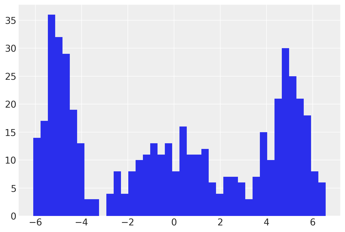
首先，我们生成一些模拟观测数据。

../_images/1c7c5303d6f30869cfe061a28ff09060db0019f1c0c5f73bad0d4a60deba0e39.png

在 PyMC 模型中，我们将为 3 个聚类中的每一个估计一个 \(\mu\) 和一个 \(\sigma\)。使用 pm.NormalMixture 分布编写高斯混合模型非常容易。

with pm.Model(coords={"cluster": range(k)}) as model:
    μ = pm.Normal(
        "μ",
        mu=0,
        sigma=5,
        transform=pm.distributions.transforms.univariate_ordered,
        initval=[-4, 0, 4],
        dims="cluster",
    )
    σ = pm.HalfNormal("σ", sigma=1, dims="cluster")
    weights = pm.Dirichlet("w", np.ones(k), dims="cluster")
    pm.NormalMixture("x", w=weights, mu=μ, sigma=σ, observed=x)

pm.model_to_graphviz(model)

../_images/57710ffc7a2372d77a0a5667fa7b19ff7dc471b78ef96565e319f5f1266fd522.svg

with model:
    idata = pm.sample()

Auto-assigning NUTS sampler...
Initializing NUTS using jitter+adapt_diag...
Multiprocess sampling (4 chains in 4 jobs)
NUTS: [μ, σ, w]

100.00% [8000/8000 00:03<00:00 Sampling 4 chains, 0 divergences]

Sampling 4 chains for 1_000 tune and 1_000 draw iterations (4_000 + 4_000 draws total) took 4 seconds.

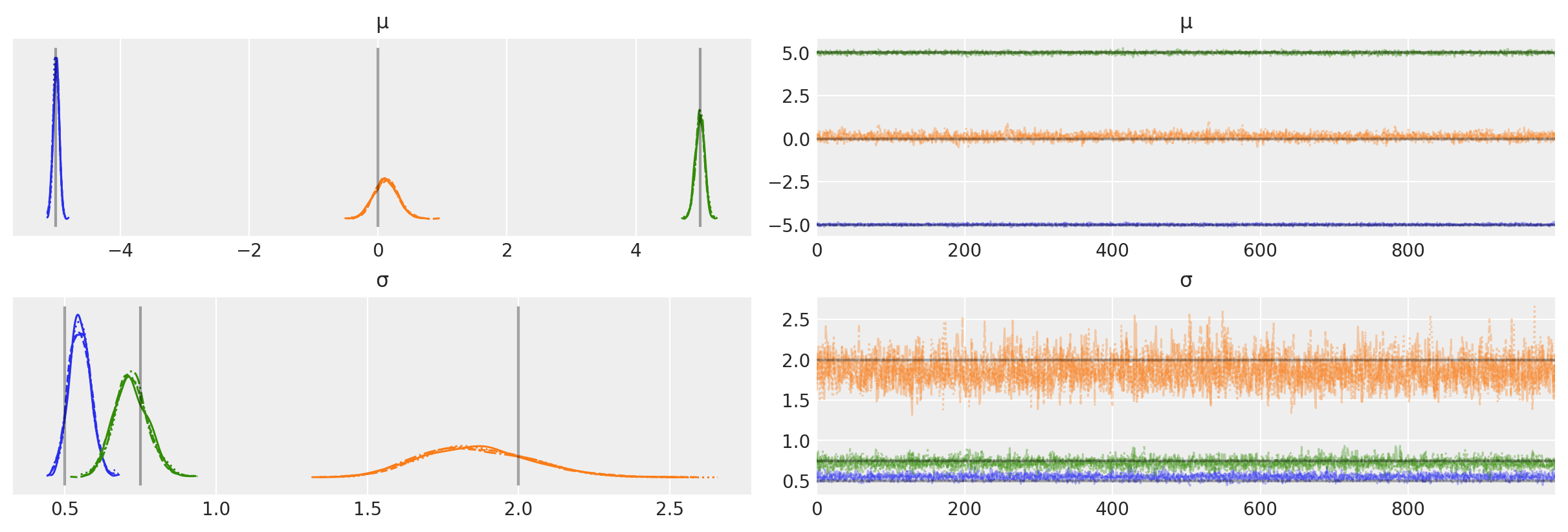
我们还可以绘制迹图以检查 MCMC 链的性质，并与真实值进行比较。

az.plot_trace(idata, var_names=["μ", "σ"], lines=[("μ", {}, [centers]), ("σ", {}, [sds])]);

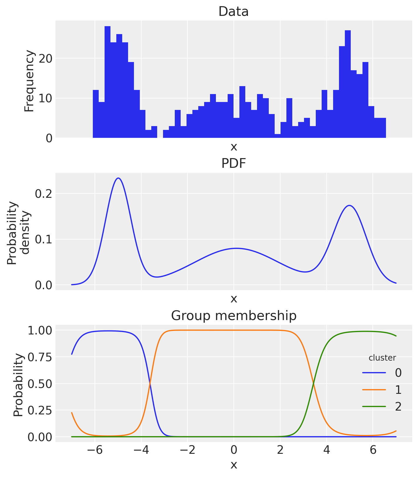
../_images/012f9879fa47ef8c3b5e07ce603bda73e12e36c99842002efbd74094d1b5beff.png

如果我们愿意，我们还可以计算概率密度函数，并根据后验均值估计检查估计的组成员概率。

xi = np.linspace(-7, 7, 500)
post = idata.posterior
pdf_components = XrContinuousRV(norm, post["μ"], post["σ"]).pdf(xi) * post["w"]
pdf = pdf_components.sum("cluster")

fig, ax = plt.subplots(3, 1, figsize=(7, 8), sharex=True)
# empirical histogram
ax[0].hist(x, 50)
ax[0].set(title="Data", xlabel="x", ylabel="Frequency")
# pdf
pdf_components.mean(dim=["chain", "draw"]).sum("cluster").plot.line(ax=ax[1])
ax[1].set(title="PDF", xlabel="x", ylabel="Probability\ndensity")
# plot group membership probabilities
(pdf_components / pdf).mean(dim=["chain", "draw"]).plot.line(hue="cluster", ax=ax[2])
ax[2].set(title="Group membership", xlabel="x", ylabel="Probability");

../_images/be9b6ee2d6c50c4472ef2968ae6fab25860073371be2aa29ebade1adf9952628.png

作者#

由 Abe Flaxman 编写。
由 Thomas Wiecki 更新。
由 Benjamin T. Vincent 于 2022 年 4 月更新 (#310)，以使用 pm.NormalMixture。
由 Benjamin T. Vincent 于 2023 年 2 月更新，以在 PyMC v5 上运行。

水印#

%load_ext watermark
%watermark -n -u -v -iv -w -p pytensor,aeppl,xarray,xarray_einstats

Last updated: Wed Feb 01 2023

Python implementation: CPython
Python version       : 3.11.0
IPython version      : 8.9.0

pytensor       : 2.8.11
aeppl          : not installed
xarray         : 2023.1.0
xarray_einstats: 0.5.1

pymc      : 5.0.1
arviz     : 0.14.0
numpy     : 1.24.1
pandas    : 1.5.3
matplotlib: 3.6.3

Watermark: 2.3.1

许可声明#

本示例库中的所有 notebook 均在 MIT 许可证下提供，该许可证允许修改和再分发用于任何用途，前提是保留版权和许可声明。

引用 PyMC 示例#

要引用此 notebook，请使用 Zenodo 为 pymc-examples 存储库提供的 DOI。

重要提示

许多 notebook 改编自其他来源：博客、书籍…… 在这种情况下，您也应该引用原始来源。

另请记住引用您的代码使用的相关库。

这是一个 bibtex 引用模板

@incollection{citekey,
  author    = "<notebook authors, see above>",
  title     = "<notebook title>",
  editor    = "PyMC Team",
  booktitle = "PyMC examples",
  doi       = "10.5281/zenodo.5654871"
}

渲染后可能如下所示

分类

标签

高斯混合模型#

作者#

水印#

许可声明#

引用 PyMC 示例#