%matplotlib inline
import arviz as az
import matplotlib.pyplot as plt
import numpy as np
import pymc3 as pm
import theano

from pymc3.ode import DifferentialEquation
from scipy.integrate import odeint

plt.style.use("seaborn-darkgrid")
GSoC 2019:pymc3.ode API 介绍#
常微分方程 (ODE) 是一个方便的数学框架,用于建模从工程学到生态学等学科中系统的时序动态。尽管大多数分析侧重于不动点的分岔和稳定性,但在实际应用系统中,如群体药代动力学和药效动力学,参数和不确定性估计更为重要。
参数估计和不确定性传播都可以通过贝叶斯框架优雅地处理。在本笔记本中,我展示了如何使用 PyMC3 中的 ode 子模块对微分方程进行推断。虽然当前的实现非常灵活且集成良好,但更复杂的模型可能很容易变得难以估计。一个新的软件包 sunode 将更快的 sundials 包集成到 PyMC3 中,可以在这里找到。
微分方程回顾#
微分方程是描述未知函数的导数与其自身关系的方程。我们通常将微分方程写成:
这里,\(\mathbf{y}\) 是未知函数,\(t\) 是时间,\(\mathbf{p}\) 是参数向量。函数 \(f\) 可以是标量值或向量值。
只有少数微分方程具有解析解。对于大多数应用领域中感兴趣的微分方程,必须使用数值方法来获得近似解。
使用微分方程进行贝叶斯推断#
PyMC3 使用哈密顿蒙特卡洛 (HMC) 从后验分布中获取样本。HMC 需要 ODE 解对参数 \(p\) 的导数。ode 子模块会自动计算适当的导数,因此您无需手动计算。您只需要:
将微分方程编写为 Python 函数
在 PyMC3 中编写模型
点击推断按钮 \(^{\text{TM}}\)
让我们通过一个小例子来看看如何在实践中完成。
自由落体的微分方程#
一个质量为 \(m\) 的物体被带到一定高度,并允许其自由下落直至地面。描述物体随时间速度变化的微分方程是:
物体在向下方向上受到的力是 \(mg\),而物体在相反方向上受到的力(由于空气阻力)与物体当前移动的速度成正比。让我们假设物体从静止开始(即物体的初始速度为 0)。情况可能并非如此。为了展示如何对初始条件进行推断,我将首先假设物体从静止开始,然后再放宽这个假设。
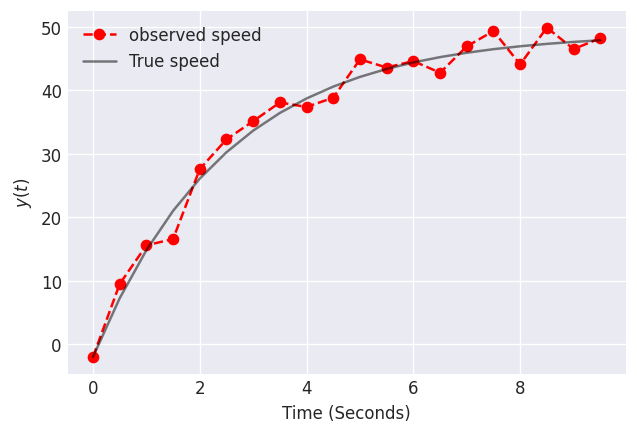
下面显示了该物体速度随时间变化的数据。数据可能由于我们的测量工具而存在噪声,或者由于物体形状不规则,从而导致自由落体过程中物体在不同时间空气动力学性能不同。让我们使用这些数据来估计空气阻力的比例常数。
# For reproducibility
np.random.seed(20394)


def freefall(y, t, p):
    return 2.0 * p[1] - p[0] * y[0]


# Times for observation
times = np.arange(0, 10, 0.5)
gamma, g, y0, sigma = 0.4, 9.8, -2, 2
y = odeint(freefall, t=times, y0=y0, args=tuple([[gamma, g]]))
yobs = np.random.normal(y, 2)

fig, ax = plt.subplots(dpi=120)
plt.plot(times, yobs, label="observed speed", linestyle="dashed", marker="o", color="red")
plt.plot(times, y, label="True speed", color="k", alpha=0.5)
plt.legend()
plt.xlabel("Time (Seconds)")
plt.ylabel(r"$y(t)$")
plt.show()
要使用 pyMC3 指定常微分方程,请使用 DifferentialEquation 类。此类接受以下参数
func:指定微分方程的函数(即 \(f(\mathbf{y},t,\mathbf{p})\))。times:观测到数据的时间数组。n_states:\(f(\mathbf{y},t,\mathbf{p})\) 的维度。n_theta:\(\mathbf{p}\) 的维度。t0:可选时间,初始条件属于该时间。
参数 func 需要编写成好像 y 和 p 是向量一样。因此,即使您的模型只有一个状态和/或一个参数,您也应该显式地写 y[0] 和/或 p[0]。
一旦模型被指定,我们可以通过传递参数和初始条件在我们的 pyMC3 模型中使用它。DifferentialEquation 返回一个扁平化的解,因此您需要将其重塑为与模型中观测数据相同的形状。
下面显示的是一个用于估计上述 ODE 中 \(\gamma\) 的模型。
ode_model = DifferentialEquation(func=freefall, times=times, n_states=1, n_theta=2, t0=0)

with pm.Model() as model:
    # Specify prior distributions for some of our model parameters
    sigma = pm.HalfCauchy("sigma", 1)
    gamma = pm.Lognormal("gamma", 0, 1)

    # If we know one of the parameter values, we can simply pass the value.
    ode_solution = ode_model(y0=[0], theta=[gamma, 9.8])
    # The ode_solution has a shape of (n_times, n_states)

    Y = pm.Normal("Y", mu=ode_solution, sigma=sigma, observed=yobs)

    prior = pm.sample_prior_predictive()
    trace = pm.sample(2000, tune=1000, cores=1)
    posterior_predictive = pm.sample_posterior_predictive(trace)

    data = az.from_pymc3(trace=trace, prior=prior, posterior_predictive=posterior_predictive)
Auto-assigning NUTS sampler...
Initializing NUTS using jitter+adapt_diag...
Sequential sampling (2 chains in 1 job)
NUTS: [gamma, sigma]
Sampling 2 chains for 1_000 tune and 2_000 draw iterations (2_000 + 4_000 draws total) took 682 seconds.
az.plot_posterior(data);
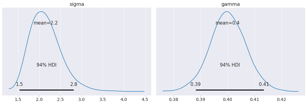
我们对比例常数和系统中噪声的估计非常接近它们的实际值!
我们甚至可以通过为其指定先验来估计重力加速度。
with pm.Model() as model2:
    sigma = pm.HalfCauchy("sigma", 1)
    gamma = pm.Lognormal("gamma", 0, 1)
    # A prior on the acceleration due to gravity
    g = pm.Lognormal("g", pm.math.log(10), 2)

    # Notice now I have passed g to the odeparams argument
    ode_solution = ode_model(y0=[0], theta=[gamma, g])

    Y = pm.Normal("Y", mu=ode_solution, sigma=sigma, observed=yobs)

    prior = pm.sample_prior_predictive()
    trace = pm.sample(2000, tune=1000, target_accept=0.9, cores=1)
    posterior_predictive = pm.sample_posterior_predictive(trace)

    data = az.from_pymc3(trace=trace, prior=prior, posterior_predictive=posterior_predictive)
Auto-assigning NUTS sampler...
Initializing NUTS using jitter+adapt_diag...
Sequential sampling (2 chains in 1 job)
NUTS: [g, gamma, sigma]
Sampling 2 chains for 1_000 tune and 2_000 draw iterations (2_000 + 4_000 draws total) took 2595 seconds.
az.plot_posterior(data);
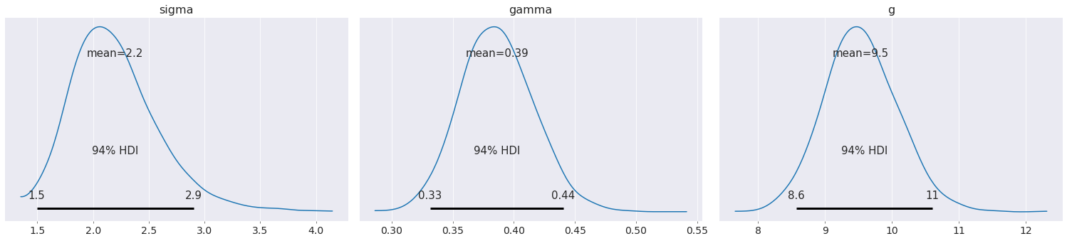
重力加速度的不确定性增加了我们对比例常数的不确定性。
最后,我们可以对初始条件进行推断。如果这个物体是被飞机带到初始高度的,那么湍流可能会使飞机上下移动,从而改变物体的初始速度。
对初始条件进行推断就像为初始条件指定先验,然后将初始条件传递给 ode_model 一样简单。
with pm.Model() as model3:
    sigma = pm.HalfCauchy("sigma", 1)
    gamma = pm.Lognormal("gamma", 0, 1)
    g = pm.Lognormal("g", pm.math.log(10), 2)
    # Initial condition prior.  We think it is at rest, but will allow for perturbations in initial velocity.
    y0 = pm.Normal("y0", 0, 2)

    ode_solution = ode_model(y0=[y0], theta=[gamma, g])

    Y = pm.Normal("Y", mu=ode_solution, sigma=sigma, observed=yobs)

    prior = pm.sample_prior_predictive()
    trace = pm.sample(2000, tune=1000, target_accept=0.9, cores=1)
    posterior_predictive = pm.sample_posterior_predictive(trace)

    data = az.from_pymc3(trace=trace, prior=prior, posterior_predictive=posterior_predictive)
Auto-assigning NUTS sampler...
Initializing NUTS using jitter+adapt_diag...
Sequential sampling (2 chains in 1 job)
NUTS: [y0, g, gamma, sigma]
/env/miniconda3/lib/python3.7/site-packages/scipy/integrate/odepack.py:248: ODEintWarning: Illegal input detected (internal error). Run with full_output = 1 to get quantitative information.
  warnings.warn(warning_msg, ODEintWarning)
Sampling 2 chains for 1_000 tune and 2_000 draw iterations (2_000 + 4_000 draws total) took 3550 seconds.
az.plot_posterior(data, figsize=(13, 3));
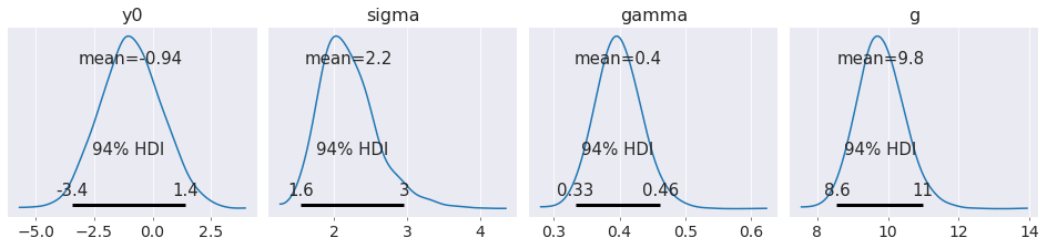
请注意,通过显式地建模初始条件,我们获得了比坚持物体从静止开始时更准确的重力加速度估计。
非线性微分方程#
自由落体物体的例子可能不是最合适的,因为那个微分方程可以精确求解。因此,不需要 DifferentialEquation 来解决那个特定的问题。然而,有很多微分方程无法精确求解。对于这些模型的推断是 DifferentialEquation 真正擅长的地方。
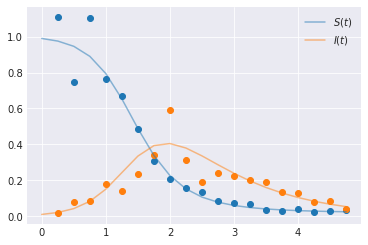
考虑 SIR 感染模型。该模型描述了疾病在均匀混合的封闭人群中传播的时序动态。人群成员被分为三种类别之一:易感者 (Susceptible)、感染者 (Infective) 或康复者 (Recovered)。微分方程如下…
约束条件是 \(S(t) + I(t) + R(t) = 1 \, \forall t\)。这里,\(\beta\) 是每位易感者和每位感染者的感染率,\(\lambda\) 是康复率。
如果我们知道 \(S(t)\) 和 \(I(t)\),那么我们可以确定 \(R(t)\),因此我们可以剥离 \(R(t)\) 的微分方程,只处理前两个方程。
在 SIR 模型中,很容易看出 \(\beta, \gamma\) 和 \(\beta/2, \gamma/2\) 将产生相同的定性动态,但时间尺度差异很大。为了研究动态的质量,而不考虑时间尺度,应用数学家将无量纲化微分方程。无量纲化是将无量纲变量引入微分方程的过程,以了解系统在等效参数化族下的动态。
为了对该系统进行无量纲化,让我们将时间缩放 \(1/\lambda\) 倍(我们这样做是因为人们平均感染时间为 \(1/\lambda\) 单位时间。这是一个直接的论证来证明这一点。更多信息,请参见 [1])。设 \(t = \tau/\lambda\),其中 \(\tau\) 是一个无量纲变量。那么…
和
量 \(\beta/\lambda\) 有一个非常特殊的名称。我们称之为 基本再生数 (\(\mathcal{R}_0\))。它的解释是,如果我们将一个感染者放入易感人群中,我们预计会出现 \(\mathcal{R}_0\) 个新的感染。如果 \(\mathcal{R}_0>1\),那么就会发生流行病。如果 \(\mathcal{R}_0\leq1\),那么就不会发生流行病(注意,我们可以通过研究系统雅可比矩阵的特征值来更严格地证明这一点。更多信息,请参见 [2])。
这种无量纲化很重要,因为它为我们提供了有关参数的信息。如果我们看到已经发生了流行病,那么我们知道 \(\mathcal{R}_0>1\),这意味着 \(\beta> \lambda\)。此外,由于 beta 的解释,可能很难对 \(\beta\) 设置先验。但是由于 \(1/\lambda\) 具有简单的解释,并且由于 \(\mathcal{R}_0>1\),我们可以通过计算 \(\mathcal{R}_0\lambda\) 来获得 \(\beta\)。
旁注:我将选择一个肯定违反这些约束的似然函数,只是为了演示如何使用 DifferentialEquation。实际上,应该选择尊重这些约束的似然函数。
def SIR(y, t, p):
    ds = -p[0] * y[0] * y[1]
    di = p[0] * y[0] * y[1] - p[1] * y[1]
    return [ds, di]


times = np.arange(0, 5, 0.25)

beta, gamma = 4, 1.0
# Create true curves
y = odeint(SIR, t=times, y0=[0.99, 0.01], args=((beta, gamma),), rtol=1e-8)
# Observational model.  Lognormal likelihood isn't appropriate, but we'll do it anyway
yobs = np.random.lognormal(mean=np.log(y[1::]), sigma=[0.2, 0.3])

plt.plot(times[1::], yobs, marker="o", linestyle="none")
plt.plot(times, y[:, 0], color="C0", alpha=0.5, label=f"$S(t)$")
plt.plot(times, y[:, 1], color="C1", alpha=0.5, label=f"$I(t)$")
plt.legend()
plt.show()
sir_model = DifferentialEquation(
    func=SIR,
    times=np.arange(0.25, 5, 0.25),
    n_states=2,
    n_theta=2,
    t0=0,
)

with pm.Model() as model4:
    sigma = pm.HalfCauchy("sigma", 1, shape=2)

    # R0 is bounded below by 1 because we see an epidemic has occurred
    R0 = pm.Bound(pm.Normal, lower=1)("R0", 2, 3)
    lam = pm.Lognormal("lambda", pm.math.log(2), 2)
    beta = pm.Deterministic("beta", lam * R0)

    sir_curves = sir_model(y0=[0.99, 0.01], theta=[beta, lam])

    Y = pm.Lognormal("Y", mu=pm.math.log(sir_curves), sigma=sigma, observed=yobs)

    trace = pm.sample(2000, tune=1000, target_accept=0.9, cores=1)
    data = az.from_pymc3(trace=trace)
Auto-assigning NUTS sampler...
Initializing NUTS using jitter+adapt_diag...
Sequential sampling (2 chains in 1 job)
NUTS: [lambda, R0, sigma]
Sampling 2 chains for 1_000 tune and 2_000 draw iterations (2_000 + 4_000 draws total) took 5339 seconds.
az.plot_posterior(data, round_to=2, credible_interval=0.95);
/dependencies/arviz/arviz/utils.py:654: UserWarning: Keyword argument credible_interval has been deprecated Please replace with hdi_prob
  ("Keyword argument credible_interval has been deprecated " "Please replace with hdi_prob"),
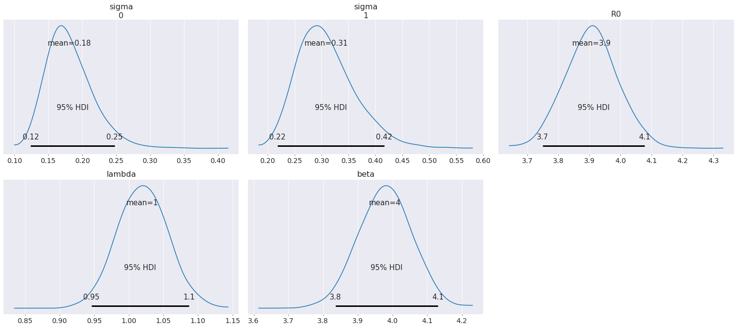
从后验图可以看出,通过利用关于无量纲参数 \(\mathcal{R}_0\) 和 \(\lambda\) 的知识,可以很好地估计 \(\beta\)。
结论与最终思考#
ODE 是连续时间演化的一个非常好的模型。随着 PyMC3 中 DifferentialEquation 的加入,我们现在可以使用贝叶斯方法来估计 ODE 的参数。
与 Stan 的 integrate_ode_bdf 相比,DifferentialEquation 速度较慢。然而,DifferentialEquation 的易用性将使从业者能够比 Stan(学习曲线陡峭)更快地开始使用贝叶斯方法估计 ODE。
参考文献#
Earn, D. J., et al. 数学流行病学. Berlin: Springer, 2008.
Britton, Nicholas F. 基础数学生物学. Springer Science & Business Media, 2012.
%load_ext watermark
%watermark -n -u -v -iv -w
arviz  0.8.3
theano 1.0.4
pymc3  3.9.0
numpy  1.18.5
last updated: Mon Jun 15 2020

CPython 3.7.7
IPython 7.15.0
watermark 2.0.2