%load_ext autoreload
%autoreload 2

import os

os.environ["THEANO_FLAGS"] = "floatX=float64"

import logging

import arviz
import matplotlib.pyplot as plt
import numpy as np
import pymc3 as pm
import theano
import theano.tensor as tt

from scipy.integrate import odeint

# this notebook show DEBUG log messages
logging.getLogger("pymc3").setLevel(logging.DEBUG)

import IPython.display

pymc3.ode：形状和基准测试

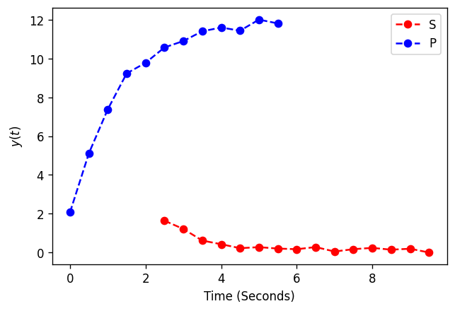
演示场景：简单的酶促反应

该模型共有两个 ODE 和 3 个参数。

在我们生成的数据中，我们将观察不同时间点的 S 和 P，以演示如何在这些情况下进行切片。

# For reproducibility
np.random.seed(23489)


class Chem:
    @staticmethod
    def reaction(y, t, p):
        S, P = y[0], y[1]
        vmax, K_S = p[0], p[1]
        dPdt = vmax * (S / K_S + S)
        dSdt = -dPdt
        return [
            dSdt,
            dPdt,
        ]


# Times for observation
times = np.arange(0, 10, 0.5)
red = np.arange(5, len(times))
blue = np.arange(12)
x_obs_1 = times[red]
x_obs_2 = times[blue]

y0_true = (10, 2)
theta_true = vmax, K_S = (0.5, 2)
sigma = 0.2

y_obs = odeint(Chem.reaction, t=times, y0=y0_true, args=(theta_true,))
y_obs_1 = np.random.normal(y_obs[red, 0], sigma)
y_obs_2 = np.random.normal(y_obs[blue, 1], sigma)

fig, ax = plt.subplots(dpi=120)
plt.plot(x_obs_1, y_obs_1, label="S", linestyle="dashed", marker="o", color="red")
plt.plot(x_obs_2, y_obs_2, label="P", linestyle="dashed", marker="o", color="blue")
plt.legend()
plt.xlabel("Time (Seconds)")
plt.ylabel(r"$y(t)$")
plt.show()

# To demonstrate that test-value computation works, but also for debugging
theano.config.compute_test_value = "raise"
theano.config.exception_verbosity = "high"
theano.config.traceback.limit = 100

def get_model():
    with pm.Model() as pmodel:
        sigma = pm.HalfCauchy("sigma", 1)
        vmax = pm.Lognormal("vmax", 0, 1)
        K_S = pm.Lognormal("K_S", 0, 1)
        s0 = pm.Normal("red_0", mu=10, sigma=2)

        y_hat = pm.ode.DifferentialEquation(
            func=Chem.reaction, times=times, n_states=len(y0_true), n_theta=len(theta_true)
        )(y0=[s0, y0_true[1]], theta=[vmax, K_S], return_sens=False)

        red_hat = y_hpt.T[0][red]
        blue_hat = y_hpt.T[1][blue]

        Y_red = pm.Normal("Y_red", mu=red_hat, sigma=sigma, observed=y_obs_1)
        Y_blue = pm.Normal("Y_blue", mu=blue_hat, sigma=sigma, observed=y_obs_2)

    return pmodel


def make_benchmark():
    pmodel = get_model()

    # select input variables & test values
    t_inputs = pmodel.cont_vars
    # apply transformations as required
    test_inputs = (np.log(0.2), np.log(0.5), np.log(1.9), 10)

    # create a test function for evaluating the logp value
    print("Compiling f_logpt")
    f_logpt = theano.function(
        inputs=t_inputs,
        outputs=[pmodel.logpt],
        # with float32, allow downcast because the forward integration is always float64
        allow_input_downcast=(theano.config.floatX == "float32"),
    )
    print(f"Test logpt:")
    print(f_logpt(*test_inputs))

    # and another test function for evaluating the gradient
    print("Compiling f_logpt")
    f_grad = theano.function(
        inputs=t_inputs,
        outputs=tt.grad(pmodel.logpt, t_inputs),
        # with float32, allow downcast because the forward integration is always float64
        allow_input_downcast=(theano.config.floatX == "float32"),
    )
    print(f"Test gradient:")
    print(f_grad(*test_inputs))

    # make a benchmarking function that uses random inputs
    # - to avoid cheating by caching
    # - to get a more realistic distribution over simulation times
    def bm():
        f_grad(
            np.log(np.random.uniform(0.1, 0.2)),
            np.log(np.random.uniform(0.4, 0.6)),
            np.log(np.random.uniform(1.9, 2.1)),
            np.random.uniform(9, 11),
        )

    return pmodel, bm

model, benchmark = make_benchmark()

print("\nPerformance:")
%timeit benchmark()

Applied log-transform to sigma and added transformed sigma_log__ to model.
Applied log-transform to vmax and added transformed vmax_log__ to model.
Applied log-transform to K_S and added transformed K_S_log__ to model.
make_node for inputs -5657601466326543627

Compiling f_logpt
Test logpt:
[array(5.73420592)]
Compiling f_logpt

grad w.r.t. inputs -5657601466326543627

Test gradient:
[array(-12.25120609), array(26.04782273), array(-9.38484546), array(11.26454126)]

Performance:
23.7 ms ± 429 µs per loop (mean ± std. dev. of 7 runs, 10 loops each)

检查计算图

如果您放大顶部的大的 DifferentialEquation 椭圆，您可以沿着蓝色箭头向下查看，以了解梯度直接从原始的 DifferentialEquation Op 节点传递。

theano.printing.pydotprint(tt.grad(model.logpt, model.vmax), "ODE_API_shapes_and_benchmarking.png")
IPython.display.Image("ODE_API_shapes_and_benchmarking.png")

grad w.r.t. inputs -5657601466326543627

The output file is available at ODE_API_shapes_and_benchmarking.png

使用下面的单元格，您可以交互式地可视化计算图。（HTML 文件保存在此 notebook 旁边。）

如果您需要安装 graphviz/pydot，您可以使用以下命令

conda install -c conda-forge python-graphviz
pip install pydot

from theano import d3viz

d3viz.d3viz(model.logpt, "ODE_API_shapes_and_benchmarking.html")

%load_ext watermark
%watermark -n -u -v -iv -w

numpy   1.18.5
pymc3   3.9.0
theano  1.0.4
logging 0.5.1.2
IPython 7.15.0
arviz   0.8.3
last updated: Sat Jun 13 2020 

CPython 3.7.7
IPython 7.15.0
watermark 2.0.2