


条件自回归 (CAR) 模型用于空间数据#
import os

import arviz as az
import matplotlib.pyplot as plt
import numpy as np
import pandas as pd
import pymc as pm
import pytensor.tensor as pt
注意
此 notebook 使用的库不是 PyMC 的依赖项,因此需要专门安装才能运行此 notebook。打开下面的下拉菜单以获取更多指导。
额外的依赖安装说明
为了运行此 notebook(本地或在 binder 上),您不仅需要安装可用的 PyMC 以及所有可选依赖项,还需要安装一些额外的依赖项。有关安装 PyMC 本身的建议,请参阅 安装
您可以使用首选的包管理器安装这些依赖项,我们提供 pip 和 conda 命令作为示例如下。
$ pip install geopandas libpysal
请注意,如果您想(或需要)从 notebook 内部而不是命令行安装软件包,您可以通过运行 pip 命令的变体来安装软件包
import sys
!{sys.executable} -m pip install geopandas libpysal
您不应运行 !pip install,因为它可能会将软件包安装在不同的环境中,即使安装了,也无法从 Jupyter notebook 中访问。
另一种替代方法是使用 conda
$ conda install geopandas libpysal
当使用 conda 安装科学 python 软件包时,我们建议使用 conda forge
# THESE ARE THE LIBRARIES THAT ARE NOT DEPENDENCIES ON PYMC
import libpysal

from geopandas import read_file
RANDOM_SEED = 8927
rng = np.random.default_rng(RANDOM_SEED)
az.style.use("arviz-darkgrid")
条件自回归 (CAR) 模型#
一组随机效应 \(\{\phi_i\}_{i=1}^N\) 的条件自回归 CAR 先验 将随机效应 \(\phi_i\) 建模为具有均值,即观测值 \(i\) 的相邻邻居的随机效应的加权平均值。在数学上,这可以表示为
其中 \({j \sim i}\) 表示观测值 \(i\) 的相邻邻居的集合,\(n_i\) 表示观测值 \(i\) 拥有的相邻邻居的数量,\(w_{ij}\) 是观测值 \(i\) 和 \(j\) 之间空间关系的权重。如果 \(i\) 和 \(j\) 不相邻,则 \(w_{ij}=0\)。最后,\(\sigma_i^2\) 是每个区域的空间变化方差参数。请注意,需要邻接矩阵(指示邻居关系)和权重矩阵 \(\textbf{w}\)(指示空间关系的权重)等信息作为输入数据。我们推断的参数是 \(\{\phi\}_{i=1}^N, \{\sigma_i\}_{i=1}^N\) 和 \(\alpha\)。
模型规范#
在这里,我们将演示使用一个典型的例子来实现 CAR 模型:1975 年至 1980 年间苏格兰的唇癌风险数据。原始数据来自 [1]。此数据集包括在苏格兰 \(N=56\) 个空间单元中观察到的唇癌病例数 \(\{y_i\}_{i=1}^N\),以及作为偏移项的预期病例数 \(\{E_i\}_{i=1}^N\)、截距参数以及区域特定连续变量的参数,该变量表示农业、渔业或林业从业人口的比例,用 \(\{x_i\}_{i=1}^N\) 表示。我们想模拟唇癌发病率与各行业就业分布之间的关系,因为暴露在阳光下是一个风险因素。在数学上,该模型为
其中 \(a\) 是回归系数的先验分布方差的某个选定的超参数。
准备数据#
我们需要加载数据集以访问变量 \(\{y_i, x_i, E_i\}_{i=1}^N\)。但对于 CAR 模型的使用而言,更独特的是创建必要的空间邻接矩阵。对于我们拟合的模型,所有邻居的权重都为 \(1\),从而避免了对权重矩阵的需求。
try:
    df_scot_cancer = pd.read_csv(os.path.join("..", "data", "scotland_lips_cancer.csv"))
except FileNotFoundError:
    df_scot_cancer = pd.read_csv(pm.get_data("scotland_lips_cancer.csv"))
df_scot_cancer.head()
| CODENO | NAME | CANCER | CEXP | AFF | ADJ | WEIGHTS | |
|---|---|---|---|---|---|---|---|
| 0 | 6126 | 斯凯-洛哈尔什 | 9 | 1.38 | 16 | [5, 9, 11, 19] | [1, 1, 1, 1] |
| 1 | 6016 | 班夫-布肯 | 39 | 8.66 | 16 | [7, 10] | [1, 1] |
| 2 | 6121 | 凯思内斯 | 11 | 3.04 | 10 | [6, 12] | [1, 1] |
| 3 | 5601 | 伯威克郡 | 9 | 2.53 | 24 | [18, 20, 28] | [1, 1, 1] |
| 4 | 6125 | 罗斯-克罗马蒂 | 15 | 4.26 | 10 | [1, 11, 12, 13, 19] | [1, 1, 1, 1, 1] |
# observed cancer counts
y = df_scot_cancer["CANCER"].values

# number of observations
N = len(y)

# expected cancer counts E for each county: this is calculated using age-standardized rates of the local population
E = df_scot_cancer["CEXP"].values
logE = np.log(E)
# proportion of the population engaged in agriculture, forestry, or fishing
x = df_scot_cancer["AFF"].values / 10.0
以下是我们创建必要邻接矩阵的步骤,其中矩阵的条目 \(i,j\) 如果观测值 \(i\) 和 \(j\) 被认为是邻居,则为 \(1\),否则为 \(0\)。
# spatial adjacency information: column `ADJ` contains list entries which are preprocessed to obtain adj as a list of lists
adj = (
    df_scot_cancer["ADJ"].apply(lambda x: [int(val) for val in x.strip("][").split(",")]).to_list()
)
# change to Python indexing (i.e. -1)
for i in range(len(adj)):
    for j in range(len(adj[i])):
        adj[i][j] = adj[i][j] - 1
# storing the adjacency matrix as a two-dimensional np.array
adj_matrix = np.zeros((N, N), dtype="int32")

for area in range(N):
    adj_matrix[area, adj[area]] = 1
数据可视化#
空间数据建模的一个重要方面是有效地可视化数据的空间性质,以及您选择的模型是否捕获了这种空间依赖性。
我们从 libpysal 包中加载了苏格兰唇癌数据集的替代版本,用于绘图。
_ = libpysal.examples.load_example("Scotlip")
pth = libpysal.examples.get_path("scotlip.shp")
spat_df = read_file(pth)
spat_df["PROP"] = spat_df["CANCER"] / np.exp(spat_df["CEXP"])
spat_df.head()
| CODENO | AREA | PERIMETER | RECORD_ID | DISTRICT | NAME | CODE | CANCER | POP | CEXP | AFF | geometry | PROP | |
|---|---|---|---|---|---|---|---|---|---|---|---|---|---|
| 0 | 6126 | 9.740020e+08 | 184951.0 | 1 | 1 | 斯凯-洛哈尔什 | w6126 | 9 | 28324 | 1.38 | 16 | POLYGON ((214091.875 841215.188, 218829.000 83... | 2.264207 |
| 1 | 6016 | 1.461990e+09 | 178224.0 | 2 | 2 | 班夫-布肯 | w6016 | 39 | 231337 | 8.66 | 16 | POLYGON ((383866.000 865862.000, 398721.000 86... | 0.006762 |
| 2 | 6121 | 1.753090e+09 | 179177.0 | 3 | 3 | 凯思内斯 | w6121 | 11 | 83190 | 3.04 | 10 | POLYGON ((311487.000 968650.000, 320989.000 96... | 0.526184 |
| 3 | 5601 | 8.985990e+08 | 128777.0 | 4 | 4 | 伯威克郡 | w5601 | 9 | 51710 | 2.53 | 24 | POLYGON ((377180.000 672603.000, 386871.656 67... | 0.716931 |
| 4 | 6125 | 5.109870e+09 | 580792.0 | 5 | 5 | 罗斯-克罗马蒂 | w6125 | 15 | 129271 | 4.26 | 10 | POLYGON ((278680.062 882371.812, 294960.000 88... | 0.211835 |
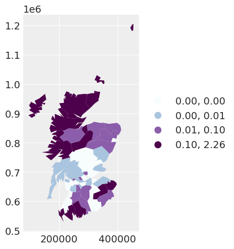
我们最初绘制每个区域的观测癌症计数与预期癌症计数的比率。我们在此图中观察到的空间依赖性表明,我们可能需要考虑数据的空间模型。
scotland_map = spat_df.plot(
    column="PROP",
    scheme="QUANTILES",
    k=4,
    cmap="BuPu",
    legend=True,
    legend_kwds={"loc": "center left", "bbox_to_anchor": (1, 0.5)},
)
在 PyMC 中编写一些模型#
我们的第一个模型:一个独立随机效应模型#
我们首先拟合一个独立的随机效应模型。我们没有对区域之间的任何空间依赖性进行建模。此模型等效于具有正态随机效应的泊松回归模型,在数学上看起来像
其中 \(\tau_\text{ind}\) 是独立随机效应精度的未知参数。\(\text{Gamma}\) 先验的值是针对我们的第二个模型选择的,因此我们将推迟解释我们的选择,直到那时。
with pm.Model(coords={"area_idx": np.arange(N)}) as independent_model:
    beta0 = pm.Normal("beta0", mu=0.0, tau=1.0e-5)
    beta1 = pm.Normal("beta1", mu=0.0, tau=1.0e-5)
    # variance parameter of the independent random effect
    tau_ind = pm.Gamma("tau_ind", alpha=3.2761, beta=1.81)

    # independent random effect
    theta = pm.Normal("theta", mu=0, tau=tau_ind, dims="area_idx")

    # exponential of the linear predictor -> the mean of the likelihood
    mu = pm.Deterministic("mu", pt.exp(logE + beta0 + beta1 * x + theta), dims="area_idx")

    # likelihood of the observed data
    y_i = pm.Poisson("y_i", mu=mu, observed=y, dims="area_idx")

    # saving the residual between the observation and the mean response for the area
    res = pm.Deterministic("res", y - mu, dims="area_idx")

    # sampling the model
    independent_idata = pm.sample(2000, tune=2000)
Auto-assigning NUTS sampler...
Initializing NUTS using jitter+adapt_diag...
Multiprocess sampling (4 chains in 4 jobs)
NUTS: [beta0, beta1, tau_ind, theta]
Sampling 4 chains for 2_000 tune and 2_000 draw iterations (8_000 + 8_000 draws total) took 32 seconds.
我们可以绘制第一个模型的残差。
spat_df["INDEPENDENT_RES"] = independent_idata["posterior"]["res"].mean(dim=["chain", "draw"])
independent_map = spat_df.plot(
    column="INDEPENDENT_RES",
    scheme="QUANTILES",
    k=5,
    cmap="BuPu",
    legend=True,
    legend_kwds={"loc": "center left", "bbox_to_anchor": (1, 0.5)},
)
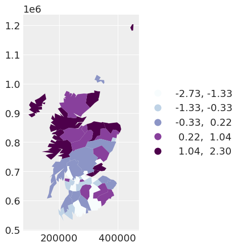
区域残差的均值似乎在空间上相关。这促使我们探索通过使用条件自回归 (CAR) 先验来添加空间相关的随机效应。
我们的第二个模型:一个空间随机效应模型(具有固定的空间依赖性)#
让我们拟合一个模型,该模型为每个区域具有两个随机效应:一个独立随机效应和一个空间随机效应。此模型看起来像
其中行 \(\phi_i \big | \mathbf{\phi}_{j\sim i} \sim \text{Normal}\big(\mu=\alpha\sum_{j=1}^{n_i}\phi_j, \tau=\tau_{\text{spat}}\big )\) 表示 CAR 先验,\(\tau_\text{spat}\) 是空间随机效应精度的未知参数,\(\alpha\) 捕获区域之间空间依赖性的程度。在本例中,我们将 \(\alpha=0.95\) 固定。
旁注: 这里我们解释了用于两个随机效应项精度的先验。由于我们对于每个 \(i\) 都有两个随机效应 \(\theta_i\) 和 \(\phi_i\),它们是独立不可识别的,但总和 \(\theta_i + \phi_i\) 是可识别的。但是,通过以这种方式缩放此精度的先验,人们可以解释每个随机效应解释的方差比例。
with pm.Model(coords={"area_idx": np.arange(N)}) as fixed_spatial_model:
    beta0 = pm.Normal("beta0", mu=0.0, tau=1.0e-5)
    beta1 = pm.Normal("beta1", mu=0.0, tau=1.0e-5)
    # variance parameter of the independent random effect
    tau_ind = pm.Gamma("tau_ind", alpha=3.2761, beta=1.81)
    # variance parameter of the spatially dependent random effects
    tau_spat = pm.Gamma("tau_spat", alpha=1.0, beta=1.0)

    # area-specific model parameters
    # independent random effect
    theta = pm.Normal("theta", mu=0, tau=tau_ind, dims="area_idx")
    # spatially dependent random effect, alpha fixed
    phi = pm.CAR("phi", mu=np.zeros(N), tau=tau_spat, alpha=0.95, W=adj_matrix, dims="area_idx")

    # exponential of the linear predictor -> the mean of the likelihood
    mu = pm.Deterministic("mu", pt.exp(logE + beta0 + beta1 * x + theta + phi), dims="area_idx")

    # likelihood of the observed data
    y_i = pm.Poisson("y_i", mu=mu, observed=y, dims="area_idx")

    # saving the residual between the observation and the mean response for the area
    res = pm.Deterministic("res", y - mu, dims="area_idx")

    # sampling the model
    fixed_spatial_idata = pm.sample(2000, tune=2000)
Auto-assigning NUTS sampler...
Initializing NUTS using jitter+adapt_diag...
Multiprocess sampling (4 chains in 4 jobs)
NUTS: [beta0, beta1, tau_ind, tau_spat, theta, phi]
Sampling 4 chains for 2_000 tune and 2_000 draw iterations (8_000 + 8_000 draws total) took 55 seconds.
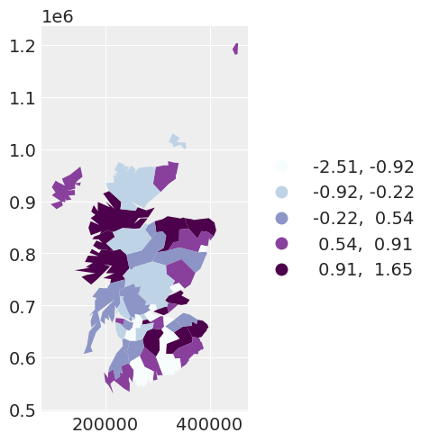
我们可以通过绘制第二个模型的残差看到,通过使用 CAR 先验考虑空间依赖性,模型的残差相对于观测值的空间位置显得更加独立。
spat_df["SPATIAL_RES"] = fixed_spatial_idata["posterior"]["res"].mean(dim=["chain", "draw"])
fixed_spatial_map = spat_df.plot(
    column="SPATIAL_RES",
    scheme="quantiles",
    k=5,
    cmap="BuPu",
    legend=True,
    legend_kwds={"loc": "center left", "bbox_to_anchor": (1, 0.5)},
)
如果我们想对我们指定的模型进行完全贝叶斯分析,我们将估计空间依赖性参数 \(\alpha\)。这将导致 ...
我们的第三个模型:一个空间随机效应模型,具有未知的空间依赖性#
模型 3 和模型 2 之间唯一的区别在于,在模型 3 中,\(\alpha\) 是未知的,因此我们对其设置了一个先验 \(\alpha \sim \text{Beta} \big (\alpha = 1, \beta=1\big )\)。
with pm.Model(coords={"area_idx": np.arange(N)}) as car_model:
    beta0 = pm.Normal("beta0", mu=0.0, tau=1.0e-5)
    beta1 = pm.Normal("beta1", mu=0.0, tau=1.0e-5)
    # variance parameter of the independent random effect
    tau_ind = pm.Gamma("tau_ind", alpha=3.2761, beta=1.81)
    # variance parameter of the spatially dependent random effects
    tau_spat = pm.Gamma("tau_spat", alpha=1.0, beta=1.0)

    # prior for alpha
    alpha = pm.Beta("alpha", alpha=1, beta=1)

    # area-specific model parameters
    # independent random effect
    theta = pm.Normal("theta", mu=0, tau=tau_ind, dims="area_idx")
    # spatially dependent random effect
    phi = pm.CAR("phi", mu=np.zeros(N), tau=tau_spat, alpha=alpha, W=adj_matrix, dims="area_idx")

    # exponential of the linear predictor -> the mean of the likelihood
    mu = pm.Deterministic("mu", pt.exp(logE + beta0 + beta1 * x + theta + phi), dims="area_idx")

    # likelihood of the observed data
    y_i = pm.Poisson("y_i", mu=mu, observed=y, dims="area_idx")

    # sampling the model
    car_idata = pm.sample(2000, tune=2000)
Auto-assigning NUTS sampler...
Initializing NUTS using jitter+adapt_diag...
Multiprocess sampling (4 chains in 4 jobs)
NUTS: [beta0, beta1, tau_ind, tau_spat, alpha, theta, phi]
Sampling 4 chains for 2_000 tune and 2_000 draw iterations (8_000 + 8_000 draws total) took 65 seconds.
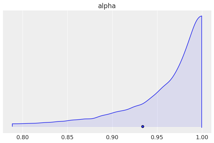
我们可以绘制 \(\alpha\) 的边际后验分布,并看到它非常接近 \(1\),表明存在很强的空间依赖性。
az.plot_density([car_idata], var_names=["alpha"], shade=0.1)
array([[<AxesSubplot: title={'center': 'alpha'}>]], dtype=object)
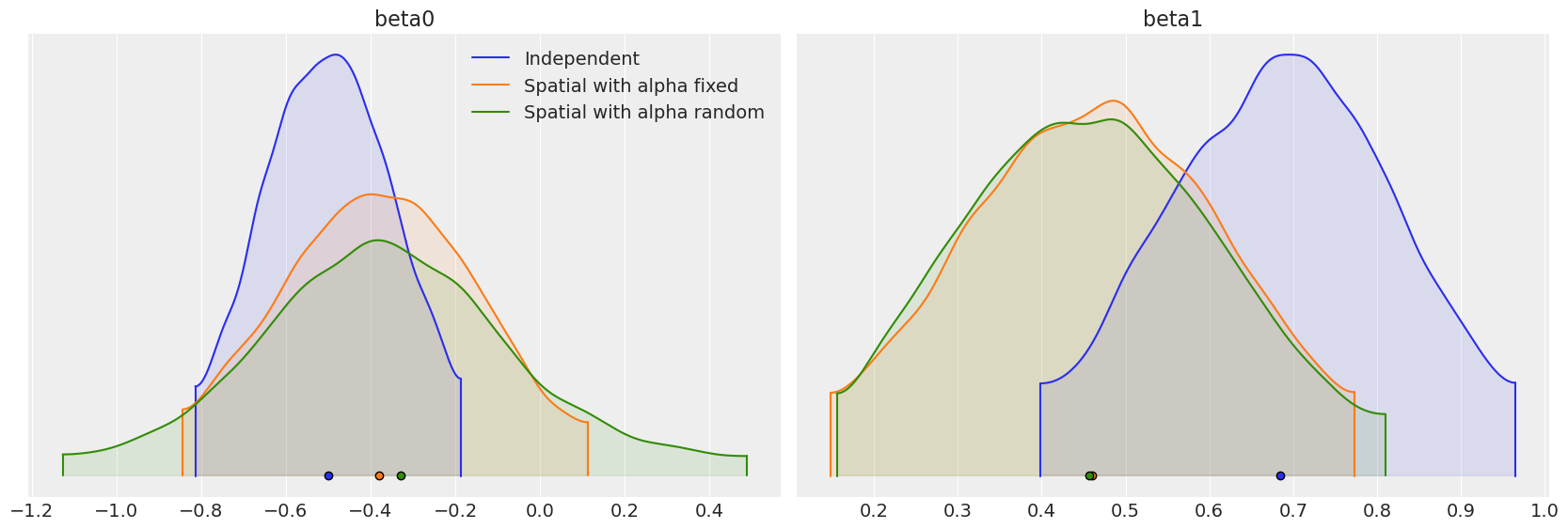
比较我们拟合的三个模型之间的回归参数 \(\beta_0\) 和 \(\beta_1\),我们可以看到,考虑观测值之间的空间依赖性可能会极大地影响对协变量对响应变量的影响的解释。
beta_density = az.plot_density(
    [independent_idata, fixed_spatial_idata, car_idata],
    data_labels=["Independent", "Spatial with alpha fixed", "Spatial with alpha random"],
    var_names=["beta0", "beta1"],
    shade=0.1,
)
局限性#
我们的最终模型提供了一些证据,表明空间依赖性参数可能为 \(1\)。但是,在 CAR 先验的定义中,\(\alpha\) 只能取到并排除 \(1\) 的值。如果 \(\alpha = 1\),我们会得到一个称为内在条件自回归 (ICAR) 先验的替代先验。ICAR 先验在空间模型中更广泛使用,特别是 BYM [Besag et al., 1991]、Leroux [Leroux et al., 2000] 和 BYM2 [Riebler et al., 2016] 模型。它还可以有效地扩展到大型数据集,这是 CAR 分布的一个局限性。目前,正在努力将 ICAR 先验包含在 PyMC 中。
参考文献#
Julian Besag、Jeremy York 和 Annie Mollié。贝叶斯图像恢复,以及空间统计中的两个应用。《统计数学研究所年报》,43(1):1–20, 1991。
Brian G Leroux、Xingye Lei 和 Norman Breslow。小区域疾病率估计:空间依赖性的新混合模型。在《流行病学、环境和临床试验中的统计模型》中,第 179–191 页。施普林格,2000 年。
Andrea Riebler、Sigrunn H Sørbye、Daniel Simpson 和 Håvard Rue。一种直观的贝叶斯空间模型,用于疾病绘图,并考虑了缩放。《医学研究统计方法》,25(4):1145–1165, 2016。
水印#
%load_ext watermark
%watermark -n -u -v -iv -w -p xarray
Last updated: Mon Jun 05 2023

Python implementation: CPython
Python version       : 3.11.0
IPython version      : 8.8.0

xarray: 2022.12.0

pymc      : 5.0.1
pytensor  : 2.8.11
pandas    : 1.5.2
numpy     : 1.24.1
arviz     : 0.14.0
libpysal  : 4.7.0
matplotlib: 3.6.2

Watermark: 2.3.1
许可证声明#
此示例库中的所有 notebook 均根据 MIT 许可证提供,该许可证允许修改和再分发以用于任何用途,前提是保留版权和许可证声明。
引用 PyMC 示例#
要引用此 notebook,请使用 Zenodo 为 pymc-examples 存储库提供的 DOI。
重要提示
许多 notebook 改编自其他来源:博客、书籍…… 在这种情况下,您也应该引用原始来源。
另请记住引用您的代码使用的相关库。
这是一个 bibtex 中的引用模板
@incollection{citekey,
  author    = "<notebook authors, see above>",
  title     = "<notebook title>",
  editor    = "PyMC Team",
  booktitle = "PyMC examples",
  doi       = "10.5281/zenodo.5654871"
}
一旦呈现,它可能看起来像