数据分叉花园#

此笔记本是 PyMC 移植的 Statistical Rethinking 2023 理查德·麦克尔里斯 (Richard McElreath) 讲座系列的一部分。

# Ignore warnings
import warnings

import arviz as az
import numpy as np
import pandas as pd
import pymc as pm
import statsmodels.formula.api as smf
import utils as utils
import xarray as xr

from matplotlib import pyplot as plt
from matplotlib import style
from scipy import stats as stats

warnings.filterwarnings("ignore")

# Set matplotlib style
STYLE = "statistical-rethinking-2023.mplstyle"
style.use(STYLE)

任务：地球表面被水覆盖的比例是多少？#

工作流程（画猫头鹰）#

定义地球仪抛掷的生成模型
定义一个 estimand – 在本例中，是地球仪被水覆盖的比例
设计一个统计程序来生成 estimand 的估计
验证统计程序 (3) 使用生成模型 – 我们可以从 (1) 生成的数据中恢复 (2) 的准确估计吗
将统计程序 (3) 应用于真实数据

1, 2. 定义地球仪抛掷的生成模型#

\(p\): 水的比例 – 这是 estimand，我们想要估计的东西
\(N\): 抛掷次数 – 我们通过实验控制这个
\(W\): 水 观测的数量
\(L\): 陆地 观测的数量

utils.draw_causal_graph(
    edge_list=[("p", "W"), ("p", "L"), ("N", "L"), ("N", "W")],
    graph_direction="LR",
    node_props={"p": {"color": "red"}},
    edge_props={("p", "W"): {"label": "influence"}},
)

../_images/8d5ab510877a4306a998a83c540e3122e298b249d447320ed49043255e4a0c7e.svg

此图定义了一个因果模型，说明 \(p, N\) 如何影响 \(W, L\) 的值。这与说它定义了一些将 \(p, N\) 映射到 \(W, L\) 值的函数 \(f\) 相同，即 \(W, L = f(p, N)\)
科学知识定义了 \(f\) 是什么或可以是什么

应用概率的朴实基础

发生方式更多的事情更合理。

贝叶斯数据分析#

“非常简单，非常谦逊”

对于样本的每一种可能的解释
计算样本可能发生的所有方式
产生观测样本的方式最多的解释更合理

3. 设计一个统计程序来生成估计#

数据分叉花园#

遵循上述口头禅…

对于每一种可能的水的比例，\(p\)
计算可能发生的所有样本抛掷方式
与更多产生样本的方式相关的 \(p\) 更合理

def calculate_n_ways_possible(observations: str, n_water: int, resolution: int = 4):
    """
    Calculate the number of ways to observing water ('W') given the toss of a globe
    with `resolution` number of sides and `n_water` faces.

    Note: this method results in numerical precision issues (due to the product) when the
    resolution of 16 or so, depending on your system.
    """
    assert n_water <= resolution

    # Convert observation string to an array
    observations = np.array(list(observations.upper()))

    # Create n-sided globe with possible outcomes
    possible = np.array(list("L" * (resolution - n_water)) + list("W" * n_water))

    # Tally up ways to obtain each observation given the possible outcomes
    # Here we use brute-force, but we could also use the analytical solution below
    ways = []
    for obs in observations:
        ways.append((possible == obs).sum())

    p_water = n_water / resolution
    # perform product in log space for numerical precision
    n_ways = np.round(np.exp(np.sum(np.log(ways)))).astype(int)
    return n_ways, p_water


def run_globe_tossing_simulation(observations, resolution, current_n_possible_ways=None):
    """Simulate the number of ways you can observe water ('W') for a globe of `resolution`
    sides, varying the proportion of the globe that is covered by water.
    """
    # For Bayesian updates
    current_n_possible_ways = (
        current_n_possible_ways if current_n_possible_ways is not None else np.array([])
    )

    print(f"Observations: '{observations}'")
    p_water = np.array([])
    for n_W in range(0, resolution + 1):
        n_L = resolution - n_W
        globe_sides = "W" * n_W + "L" * n_L
        n_possible_ways, p_water_ = calculate_n_ways_possible(
            observations, n_water=n_W, resolution=resolution
        )
        print(f"({n_W+1}) {globe_sides} p(W) = {p_water_:1.2}\t\t{n_possible_ways} Ways to Produce")

        p_water = np.append(p_water, p_water_)
        current_n_possible_ways = np.append(current_n_possible_ways, n_possible_ways)

    return current_n_possible_ways, p_water


RESOLUTION = 4
observations = "WLW"
n_possible_ways, p_water = run_globe_tossing_simulation(observations, resolution=RESOLUTION)

Observations: 'WLW'
(1) LLLL p(W) = 0.0		0 Ways to Produce
(2) WLLL p(W) = 0.25		3 Ways to Produce
(3) WWLL p(W) = 0.5		8 Ways to Produce
(4) WWWL p(W) = 0.75		9 Ways to Produce
(5) WWWW p(W) = 1.0		0 Ways to Produce

贝叶斯（在线）更新#

new_observation_possible_ways, _ = run_globe_tossing_simulation("W", resolution=RESOLUTION)

# Online update
n_possible_ways *= new_observation_possible_ways

print("\nUpdated Possibilities given new observation:")
for ii in range(0, RESOLUTION + 1):
    print(f"({ii+1}) p(W) = {p_water[ii]:1.2}\t\t{int(n_possible_ways[ii])} Ways to Produce")

Observations: 'W'
(1) LLLL p(W) = 0.0		0 Ways to Produce
(2) WLLL p(W) = 0.25		1 Ways to Produce
(3) WWLL p(W) = 0.5		2 Ways to Produce
(4) WWWL p(W) = 0.75		3 Ways to Produce
(5) WWWW p(W) = 1.0		4 Ways to Produce

Updated Possibilities given new observation:
(1) p(W) = 0.0		0 Ways to Produce
(2) p(W) = 0.25		3 Ways to Produce
(3) p(W) = 0.5		16 Ways to Produce
(4) p(W) = 0.75		27 Ways to Produce
(5) p(W) = 1.0		0 Ways to Produce

整个样本#

RESOLUTION = 4
observations = "WLWWWLWLW"
n_W = len(observations.replace("L", ""))
n_L = len(observations) - n_W

n_possible_ways, p_water = run_globe_tossing_simulation(observations, resolution=RESOLUTION)

Observations: 'WLWWWLWLW'
(1) LLLL p(W) = 0.0		0 Ways to Produce
(2) WLLL p(W) = 0.25		27 Ways to Produce
(3) WWLL p(W) = 0.5		512 Ways to Produce
(4) WWWL p(W) = 0.75		729 Ways to Produce
(5) WWWW p(W) = 1.0		0 Ways to Produce

表明我们使用解析解得到相同答案

结果表明解析解 \(W,L = (Rp)^W \times (R - Rp)^L\)#

其中 \(R\) 是可能的地球仪数量，在本例中为 4

def calculate_analytic_n_ways_possible(p, n_W, n_L, resolution=RESOLUTION):
    """This scales much better than the brute-force method"""
    return (resolution * p) ** n_W * (resolution - resolution * p) ** n_L


analytic_n_possible_ways = np.array(
    [calculate_analytic_n_ways_possible(p, n_W, n_L) for p in p_water]
)
assert (analytic_n_possible_ways == n_possible_ways).all()

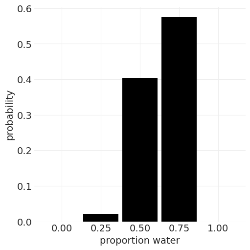
概率#

总和为 1 的非负值
通过总计数标准化大和

n_possible_probabilities = n_possible_ways / n_possible_ways.sum()

print("Proportion\tWays\tProbability")
for p, n_w, n_p in zip(p_water, n_possible_ways, n_possible_probabilities):
    print(f"{p:1.12}\t\t{n_w:0.0f}\t{n_p:1.2f}")

probs = np.linspace(0, 1, RESOLUTION + 1)
plt.subplots(figsize=(5, 5))
plt.bar(x=probs, height=n_possible_probabilities, width=0.9 / RESOLUTION, color="k")
plt.xticks(probs)
plt.ylabel("probability")
plt.xlabel("proportion water");

Proportion	Ways	Probability
0		0	0.00
25		27	0.02
5		512	0.40
75		729	0.57
0		0	0.00

../_images/1440ed3f5d13927c74fe077f7328c27245f50d6d735f474b5c810021e792065c.png

4. 使用生成模型 (1) 验证统计程序 (3)#

先测试再估计 🐤#

代码生成模拟 (1)
代码估计器 (3)
使用 (1) 测试 (3)；您应该获得预期的输出

如果你什么都不测试，你就会错过一切

4.1 生成模拟#

from pprint import pprint

np.random.seed(1)


def simulate_globe_toss(p: float = 0.7, N: int = 9) -> list[str]:
    """Simulate N globe tosses with a specific/known proportion
    p: float
        The propotion of water
    N: int
        Number of globe tosses
    """
    return np.random.choice(list("WL"), size=N, p=np.array([p, 1 - p]), replace=True)

print(simulate_globe_toss())

['W' 'L' 'W' 'W' 'W' 'W' 'W' 'W' 'W']

pprint([simulate_globe_toss(p=1, N=11).tolist() for _ in range(10)])

[['W', 'W', 'W', 'W', 'W', 'W', 'W', 'W', 'W', 'W', 'W'],
 ['W', 'W', 'W', 'W', 'W', 'W', 'W', 'W', 'W', 'W', 'W'],
 ['W', 'W', 'W', 'W', 'W', 'W', 'W', 'W', 'W', 'W', 'W'],
 ['W', 'W', 'W', 'W', 'W', 'W', 'W', 'W', 'W', 'W', 'W'],
 ['W', 'W', 'W', 'W', 'W', 'W', 'W', 'W', 'W', 'W', 'W'],
 ['W', 'W', 'W', 'W', 'W', 'W', 'W', 'W', 'W', 'W', 'W'],
 ['W', 'W', 'W', 'W', 'W', 'W', 'W', 'W', 'W', 'W', 'W'],
 ['W', 'W', 'W', 'W', 'W', 'W', 'W', 'W', 'W', 'W', 'W'],
 ['W', 'W', 'W', 'W', 'W', 'W', 'W', 'W', 'W', 'W', 'W'],
 ['W', 'W', 'W', 'W', 'W', 'W', 'W', 'W', 'W', 'W', 'W']]

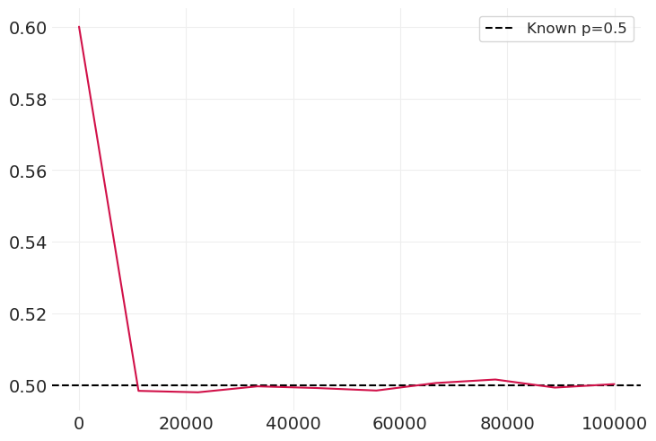
在极端设置下测试#

对于大量样本 N，估计器应收敛到已知的 \(p\)

known_p = 0.5

simulated_ps = []
sample_sizes = np.linspace(10, 100_000, 10)
for N in sample_sizes:
    simulated_p = np.sum(simulate_globe_toss(p=known_p, N=int(N)) == "W") / N
    simulated_ps.append(simulated_p)

plt.axhline(known_p, label=f"Known p={known_p}", color="k", linestyle="--")
plt.legend()
plt.plot(sample_sizes, simulated_ps);

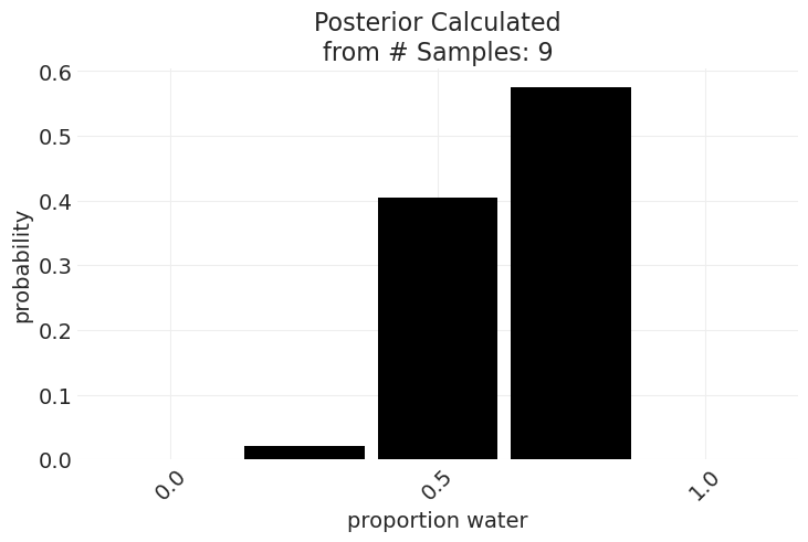
../_images/02d7bd8ccd0ca61c36d576e574506a7cba7ce7a753a82adbf7523025a3a3e802.png

4.2 编写估计器代码#

估计器接收观测值并返回潜在估计的概率分布（后验）。较高概率的估计值应该更合理。

def compute_posterior(observations, resolution=RESOLUTION, ax=None):
    n_W = len(observations.replace("L", ""))
    n_L = len(observations) - n_W

    p_water = np.linspace(0, 1, resolution + 1)
    n_possible_ways = np.array(
        [calculate_analytic_n_ways_possible(p, n_W, n_L, resolution) for p in p_water]
    )

    posterior = n_possible_ways / n_possible_ways.sum()
    potential_p = np.linspace(0, 1, resolution + 1)

    return posterior, potential_p


def plot_posterior(observations, resolution=RESOLUTION, ax=None):
    posterior, probs = compute_posterior(observations, resolution=resolution)
    if ax is not None:
        plt.sca(ax)
    plt.bar(x=probs, height=posterior, width=0.9 / resolution, color="k")
    plt.xticks(probs[::2], rotation=45)
    plt.ylabel("probability")
    plt.xlabel("proportion water")
    plt.title(f"Posterior Calculated\nfrom # Samples: {len(observations)}")


plot_posterior(observations, resolution=4)

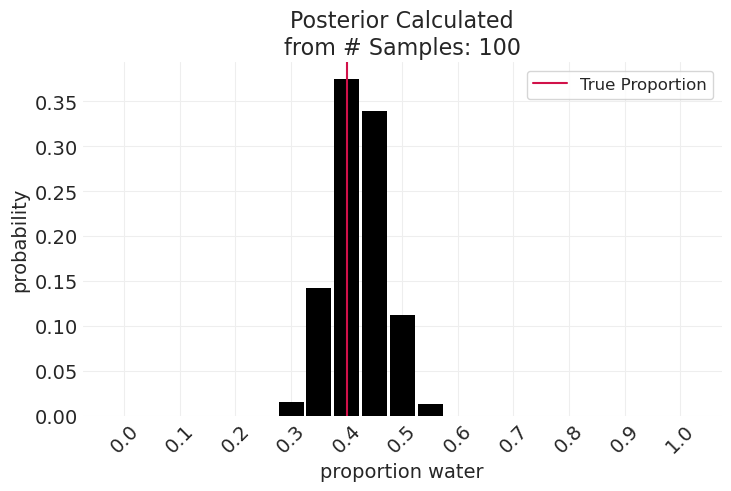
../_images/ecfe9751ff0b9effc40105960a152f5935d7b148a300325192f5be6f4c51bf03.png

np.random.seed(2)
known_p = 0.4
simulated_observations = "".join(simulate_globe_toss(p=known_p, N=100))
plot_posterior(simulated_observations, resolution=20)
plt.axvline(known_p, color="C0", label="True Proportion")
plt.legend();

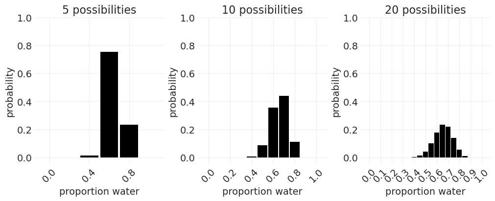
../_images/3221173d1b16dca3598579bd93dd0820e3c2f9bde46c5ad1658c3a14be2d35ec.png

无限的可能性#

从 N 面地球仪移动到无限面地球仪。#

随着我们增加地球仪的分辨率

沿着比例轴有更多的条/更精细的分辨率
条形图随着可能性的增加而变短 – 它们必须总和为 1

np.random.seed(12)
known_p = 0.7
simulated_observations = "".join(simulate_globe_toss(p=known_p, N=30))
_, axs = plt.subplots(1, 3, figsize=(10, 4))
for ii, possibilities in enumerate([5, 10, 20]):
    plot_posterior(simulated_observations, resolution=possibilities, ax=axs[ii])
    plt.ylim([-0.05, 1])
    axs[ii].set_title(f"{possibilities} possibilities")

../_images/ba0c66f6e251fe6ea80b0e61d33feb9bf4bcfe87be78ee4c30bae0a577f60962.png

Beta 分布#

解析函数，当可能性数量 \(\rightarrow \infty\) 时，它为我们提供 pdf

\[ p = \frac{(W + L + 1)!}{W!L!} p^W(1-p)^L \]

其中 \(\frac{(W + L + 1)!}{W!L!}\) 是一个归一化常数，使分布总和为 1

抛掷地球仪#

from scipy.special import factorial


def beta_posterior(n_W: int, n_L: int, p: float) -> float:
    """Calculates the beta posterior over proportions `p` given a set of
    `N_W` water and `N_L` land observations
    """
    return factorial(n_W + n_L + 1) / (factorial(n_W) * factorial(n_L)) * p**n_W * (1 - p) ** n_L


def plot_beta_posterior_from_observations(
    observations: str, resolution: int = 50, **plot_kwargs
) -> None:
    """Calculates and plots the beta posterior for a string of observations"""
    n_W = len(observations.replace("L", ""))
    n_L = len(observations) - n_W
    proportions = np.linspace(0, 1, resolution)

    probs = beta_posterior(n_W, n_L, proportions)
    plt.plot(proportions, probs, **plot_kwargs)
    plt.yticks([])
    plt.title(observations)


# Tossing the globe
observations = "WLWWWLWLW"
fig, axs = plt.subplots(3, 3, figsize=(8, 8))
for ii in range(9):
    ax = axs[ii // 3][ii % 3]
    plt.sca(ax)
    # Plot previous
    if ii > 0:
        plot_beta_posterior_from_observations(observations[:ii], color="k", linestyle="--")
    else:
        # First observation, no previous data
        plot_beta_posterior_from_observations("", color="k", linestyle="--")

    color = "C1" if observations[ii] == "W" else "C0"
    plot_beta_posterior_from_observations(
        observations[: ii + 1], color=color, linewidth=4, alpha=0.5
    )

    if not ii % 3:
        plt.ylabel("posterior probability")

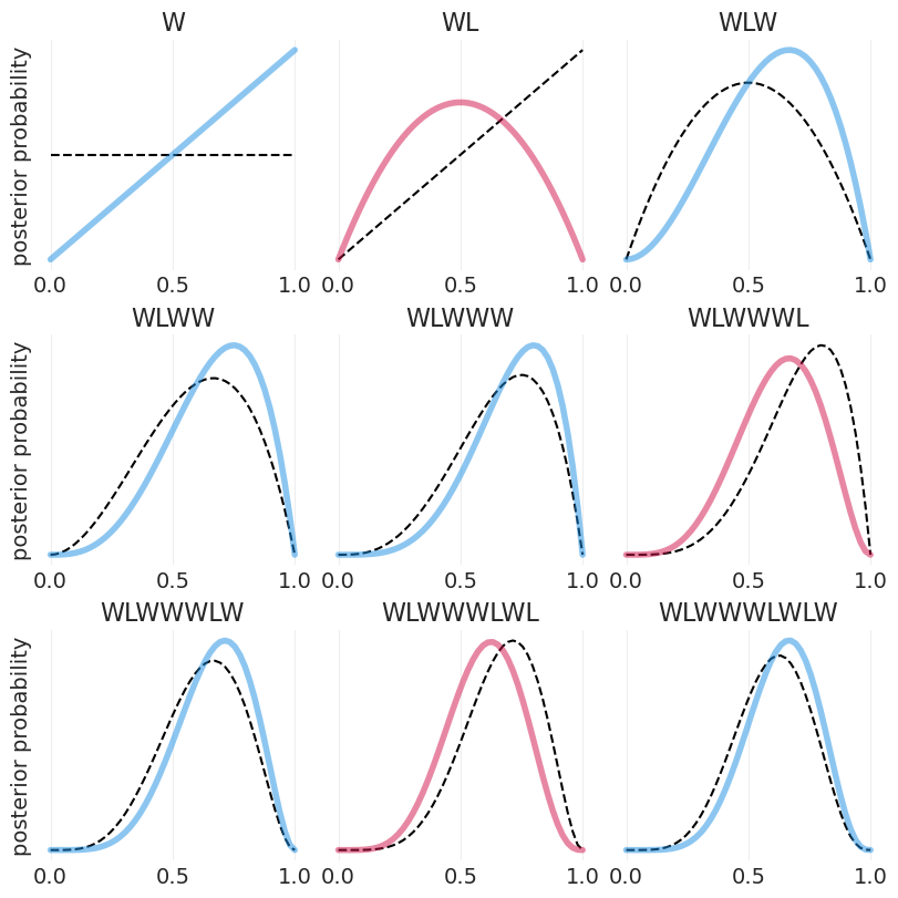
../_images/fe5f1dd5988f3ab1cf20abec330a415983f9929eb498905a588c2ebf69841644.png

关于贝叶斯推断…#

没有最小样本量 – 较少的样本会回退到先验
后验形状体现了样本大小 – 更多的数据使后验更精确
没有点估计 – 估计是整个后验分布
没有真实区间 – 可以绘制无限数量的区间，每个区间都是任意的，并且取决于您尝试沟通/总结的内容

从后验到预测#

为了进行预测，我们必须对整个后验进行平均（即积分）——这平均了后验中的不确定性
我们可以使用积分微积分来做到这一点
或者，我们可以从后验中抽取样本并对这些样本求平均值

将微积分问题变成数据摘要问题

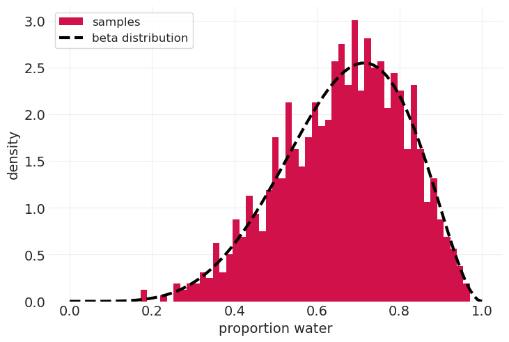
从后验分布中抽样#

a, b = 6, 3
# draw random samples from Beta PDF
beta_posterior_pdf = stats.beta(a, b)
beta_posterior_samples = beta_posterior_pdf.rvs(size=1000)

# Show that our beta postorior captures shape of beta-distributed samples
plt.hist(beta_posterior_samples, bins=50, density=True, label="samples")
probs = np.linspace(0, 1, 100)
plt.plot(
    probs,
    beta_posterior(a - 1, b - 1, probs),
    linewidth=3,
    color="k",
    linestyle="--",
    label="beta distribution",
)
plt.xlabel("proportion water")
plt.ylabel("density")
plt.legend();

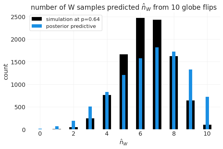
../_images/2327cbd338f9eff4bc4e403c9c097d89a5068e16bff17b36d23a6f2e176eb2df.png

从后验预测分布中抽样#

后验预测：基于当前后验估计的样本外数据预测

1. 从后验中抽取模型参数样本（即比例）
1. 使用我们的生成模型和抽样的参数生成/模拟数据预测
1. 结果概率分布就是我们的预测

# 1. Sample parameters values from posterior
N_posterior_samples = 10_000
posterior_samples = beta_posterior_pdf.rvs(size=N_posterior_samples)

# 2. Use samples for the posterior to simulate sampling 10 observations from our generative model
N_draws_for_prediction = 10
posterior_predictive = [
    (simulate_globe_toss(p, N_draws_for_prediction) == "W").sum() for p in posterior_samples
]
ppd_unique, ppd_counts = np.unique(posterior_predictive, return_counts=True)

# ...for comparison we can compare to the distribution that results from pinning the parameter to a specific value
specific_prob = 0.64
specific_predictive = [
    (simulate_globe_toss(specific_prob, N_draws_for_prediction) == "W").sum()
    for _ in posterior_samples
]
specific_unique, specific_counts = np.unique(specific_predictive, return_counts=True)

plt.bar(
    specific_unique,
    specific_counts,
    width=0.5,
    color="k",
    label=f"simulation at p={specific_prob:1.2}",
)
plt.bar(ppd_unique, ppd_counts, width=0.2, color="C1", label="posterior predictive")
plt.xlabel(r"$\hat n_W$")
plt.ylabel("count")
plt.title(f"number of W samples predicted $\hat n_W$ from {N_draws_for_prediction} globe flips")
plt.legend();

../_images/a5ecd70666a289c25a81887b6cd79c52a567808631d62a557ae34a9a1ddcbe5e.png

抽样既美观又方便#

我们将通过抽样计算的内容

预测
因果效应
反事实
先验预测

摘要：贝叶斯数据分析#

对于数据的每一种可能的解释
计算在该解释下可能发生的所有数据方式
产生数据的方式更多的解释更合理

贝叶斯谦逊#

如果你的生成模型是正确的，你就不能做得更好：这将是一个最优解
不提供保证，只提供你投入的东西

奖励：错误分类#

在之前的示例中，我们没有考虑抽样误差或测量噪声。换句话说，我们测量的 水 观测数量可能不是真实值。

这意味着 \(W\) 的真实值是未知/未测量的，但我们测量的是 \(W^*\)，它是由真实的、未测量的 \(W\) 和测量过程 \(M\) 引起的。如果我们知道我们的测量误差率，我们可以尝试对其进行建模

utils.draw_causal_graph(
    edge_list=[("p", "W"), ("W", "W*"), ("M", "W*"), ("N", "W")],
    node_props={
        "p": {"color": "red", "style": "dashed"},
        "W": {"style": "dashed", "label": "actual W"},
        "W*": {"label": "noisy W, W*"},
        "unobserved": {"style": "dashed"},
        "M": {"label": "measurement error, M"},
    },
    graph_direction="LR",
)

../_images/a11792ecb826ee6be5f69e9fc1a66947c5957bb5feb092df5acf0ea3dbf01f67.svg

错误分类模拟#

def simulate_noisy_globe_toss(p: float = 0.7, N: int = 9, error_rate: float = 0.1) -> np.ndarray:
    # True sample
    sample = np.random.choice(list("WL"), size=N, p=np.array([p, 1 - p]), replace=True)

    # Error-induced sample
    error_trials = np.random.rand(N) < error_rate
    errors_effect_sample_trials = (sample == "W") & error_trials
    sample[errors_effect_sample_trials] = "L"
    return sample


simulate_noisy_globe_toss()

array(['L', 'W', 'W', 'L', 'W', 'W', 'W', 'W', 'W'], dtype='<U1')

错误分类估计器#

def calculate_unnormalized_n_ways_possible_with_error(
    p: float, n_W: int, n_L: int, error_rate: float = 0.1
) -> float:
    n_W_error = (p * (1 - error_rate) + ((1 - p) * error_rate)) ** n_W
    n_L_error = ((1 - p) * (1 - error_rate) + (p * error_rate)) ** n_L
    return n_W_error * n_L_error


a, b = 6, 3
resolution = 100
proportions = np.linspace(0, 1, resolution)
error_rate = 0.1
error_posterior = np.array(
    [calculate_unnormalized_n_ways_possible_with_error(p, a, b, error_rate) for p in proportions]
)
beta_posterior_values = beta_posterior(a, b, proportions)

# Infer normalization constant Z directly from samples
error_posterior *= resolution / error_posterior.sum()
beta_posterior_values *= resolution / beta_posterior_values.sum()

plt.subplots(figsize=(6, 6))
plt.plot(proportions, beta_posterior_values, label="previous posterior", color="k", linewidth=4)
plt.plot(
    proportions,
    error_posterior,
    label=f"misclassification posterior\n(error rate={error_rate:1.2})",
    linewidth=4,
)
plt.xlabel("proportion of water")
plt.ylabel("posterior probability")
plt.legend();

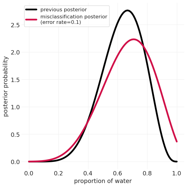
../_images/cedf6a476d0614db13e1efdfa27f1c960a4a094205d70bb09c795f466455be6a.png

测量很重要#

对测量误差建模比忽略它更好
缺失数据也是如此
重要的是样本为什么不同，以及我们明确如何对其建模

作者#

由 Dustin Stansbury (2024) 移植到 PyMC
基于 Richard McElreath 的 Statistical Rethinking (2023) 讲座

%load_ext watermark
%watermark -n -u -v -iv -w -p pytensor,aeppl,xarray

Last updated: Tue Dec 17 2024

Python implementation: CPython
Python version       : 3.12.5
IPython version      : 8.27.0

pytensor: 2.26.4
aeppl   : not installed
xarray  : 2024.7.0

numpy      : 1.26.4
scipy      : 1.14.1
matplotlib : 3.9.2
statsmodels: 0.14.2
xarray     : 2024.7.0
pymc       : 5.19.1
pandas     : 2.2.2
arviz      : 0.19.0

Watermark: 2.5.0

许可声明#

本示例 галерея 中的所有笔记本均根据 MIT 许可证提供，该许可证允许修改和再分发以用于任何用途，前提是保留版权和许可声明。

引用 PyMC 示例#

要引用此笔记本，请使用 Zenodo 为 pymc-examples 存储库提供的 DOI。

重要

许多笔记本都改编自其他来源：博客、书籍…… 在这种情况下，您也应该引用原始来源。

还请记住引用您的代码使用的相关库。

这是一个 bibtex 中的引用模板

@incollection{citekey,
  author    = "<notebook authors, see above>",
  title     = "<notebook title>",
  editor    = "PyMC Team",
  booktitle = "PyMC examples",
  doi       = "10.5281/zenodo.5654871"
}

一旦渲染，它可能看起来像

分类

标签

数据分叉花园#

任务：地球表面被水覆盖的比例是多少？#

工作流程（画猫头鹰）#

1, 2. 定义地球仪抛掷的生成模型#

贝叶斯数据分析#

3. 设计一个统计程序来生成估计#

数据分叉花园#

贝叶斯（在线）更新#

整个样本#

结果表明解析解 \(W,L = (Rp)^W \times (R - Rp)^L\)#

概率#

4. 使用生成模型 (1) 验证统计程序 (3)#

先测试再估计 🐤#

4.1 生成模拟#

在极端设置下测试#

4.2 编写估计器代码#

无限的可能性#

从 N 面地球仪移动到无限面地球仪。#

Beta 分布#

抛掷地球仪#

关于贝叶斯推断…#

从后验到预测#

从后验分布中抽样#

从后验预测分布中抽样#

抽样既美观又方便#

摘要：贝叶斯数据分析#

贝叶斯谦逊#

奖励：错误分类#

错误分类模拟#

错误分类估计器#

测量很重要#

作者#

许可声明#

引用 PyMC 示例#