


地心模型#
本 Notebook 是 Richard McElreath 的 Statistical Rethinking 2023 系列讲座的 PyMC 移植版本的一部分。
# Ignore warnings
import warnings

import arviz as az
import numpy as np
import pandas as pd
import pymc as pm
import statsmodels.formula.api as smf
import utils as utils
import xarray as xr

from matplotlib import pyplot as plt
from matplotlib import style
from scipy import stats as stats

warnings.filterwarnings("ignore")

# Set matplotlib style
STYLE = "statistical-rethinking-2023.mplstyle"
style.use(STYLE)
线性回归#
地心的
虽然总是不正确的,但却是非常好的近似
尽管是对真实现象的不准确的机制模型,但可以用作因果分析系统中的一个齿轮
高斯
通用误差模型
抽象掉细节,使我们能够进行宏观推断,而无需纳入微观现象
为什么是正态分布?#
两个论点#
生成性:总和波动趋向于正态分布(见下文)
推断性:对于估计均值和方差,在最大熵意义上,正态分布是最少信息的(最少假设)
💡 变量不需要呈正态分布,也可以使用高斯误差模型估计正确的均值和方差。
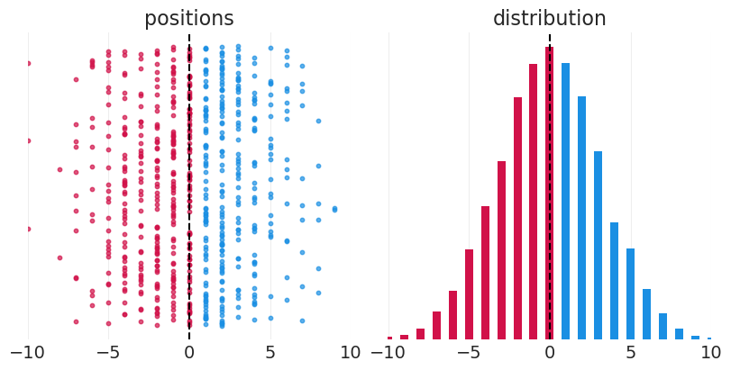
从决策的总和中生成正态分布#
模拟一群人从中心位置开始随机左右行走
最终位置是许多左右偏差的总和——结果呈正态分布
正态分布产生于偏差被求和(也包括乘积)的过程中
n_people = 10000
n_steps = 1000

step_size = 0.1
left_right_step_decisions = 2 * stats.bernoulli(p=0.5).rvs(size=(n_people, n_steps)) - 1
steps = step_size * left_right_step_decisions

positions = np.round(np.sum(steps, axis=1))
fig, axs = plt.subplots(1, 2, figsize=(8, 4))

plt.sca(axs[0])
plt.axvline(0, color="k", linestyle="--")
for ii, pos in enumerate(positions[::15]):
    color = "C1" if pos > 0 else "C0"
    plt.scatter(x=pos, y=ii, color=color, alpha=0.7, s=10)

plt.xlim([-10, 10])
plt.yticks([])
plt.title("positions")

# Plot histogram
position_unique, position_counts = np.unique(positions, return_counts=True)
positive_idx = position_unique > 0
negative_idx = position_unique <= 0
plt.sca(axs[1])
plt.bar(position_unique[positive_idx], position_counts[positive_idx], width=0.5, color="C1")
plt.bar(position_unique[negative_idx], position_counts[negative_idx], width=0.5, color="C0")
plt.axvline(0, color="k", linestyle="--")
plt.xlim([-10, 10])
plt.yticks([])
plt.title("distribution");
画猫头鹰#
阐明清晰的问题——确立一个估计量
勾勒因果假设——绘制 DAG
基于因果假设定义一个生成模型——生成合成数据
使用生成模型构建(并测试)一个估计器——我们能否恢复(3)的数据生成参数?
收益:通过分析真实数据(可能获得迭代假设、模型和/或估计器的见解)
线性回归#
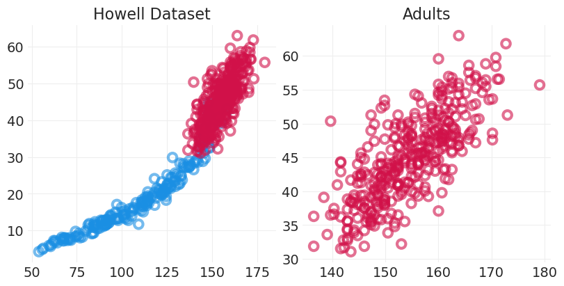
Howell 数据集#
(1)问题 & 估计量#
描述体重和身高之间的关联
我们将关注成人体重——成人身高近似线性
HOWELL = utils.load_data("Howell1")
fig, axs = plt.subplots(1, 2, figsize=(8, 4))

ADULTS = HOWELL.age >= 18
ADULT_HOWELL = HOWELL[ADULTS]
CHILD_HOWELL = HOWELL[~ADULTS]
plt.sca(axs[0])
utils.plot_scatter(CHILD_HOWELL.height, CHILD_HOWELL.weight, color="C1")
utils.plot_scatter(ADULT_HOWELL.height, ADULT_HOWELL.weight)
plt.title("Howell Dataset")

plt.sca(axs[1])
utils.plot_scatter(ADULT_HOWELL.height, ADULT_HOWELL.weight)
plt.title("Adults")
HOWELL.head()
| 身高 | 体重 | 年龄 | 男性 | |
|---|---|---|---|---|
| 0 | 151.765 | 47.825606 | 63.0 | 1 |
| 1 | 139.700 | 36.485807 | 63.0 | 0 |
| 2 | 136.525 | 31.864838 | 65.0 | 0 |
| 3 | 156.845 | 53.041914 | 41.0 | 1 |
| 4 | 145.415 | 41.276872 | 51.0 | 0 |
(2)科学模型#
身高如何影响体重?
即 “体重是身高的某个函数”
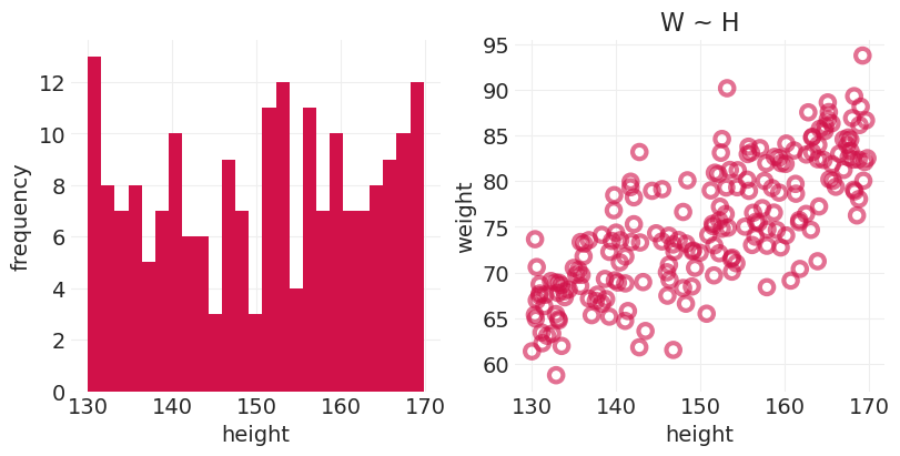
(3)生成模型#
选项
动态 - 关系随时间变化
静态 - 随时间恒定的趋势
“体重 \(W\) 是身高 \(H\) 和一些未观察到的因素 \(U\) 的函数”
utils.draw_causal_graph(
    edge_list=[("H", "W"), ("U", "W")],
    node_props={"U": {"style": "dashed"}, "unobserved": {"style": "dashed"}},
    graph_direction="LR",
)

线性回归模型#
我们需要一个函数,将成人体重映射为身高的比例加上一些未观察到/未考虑到的原因。引入线性回归
生成模型描述:#
描述模型#
左侧的变量
右侧的定义
\(\sim\) 表示从分布中抽样
例如, \(H_i \sim \text{Uniform}(130, 170)\) 是身高在 130 到 170 之间均匀分布的定义
\(=\) 表示统计期望或确定性相等
例如, \(W_i \sim \beta H_i + U_i\) 是预期体重方程的定义
下标 \(i\) 表示观察/个体的索引
通常代码将以相反的方向编写,因为您需要先定义变量才能被引用/组合
def simulate_weight(H: np.array, beta: float, sigma: float) -> np.ndarray:
    """
    Generative model describe above, simulate weight given height, `H`,
    proportional coefficient `beta`, and the standard deviation of
    unobserved (Normally-distributed) noise, sigma.
    """
    n_heights = len(H)

    # unobserved noise
    U = stats.norm.rvs(0, sigma, size=n_heights)
    return beta * H + U


n_heights = 200
MIN_HEIGHT = 130
MAX_HEIGHT = 170
H = stats.uniform.rvs(MIN_HEIGHT, MAX_HEIGHT - MIN_HEIGHT, size=n_heights)
W = simulate_weight(H, beta=0.5, sigma=5)

fig, axs = plt.subplots(1, 2, figsize=(8, 4))
plt.sca(axs[0])
plt.hist(H, bins=25)
plt.xlabel("height")
plt.ylabel("frequency")

plt.sca(axs[1])
utils.plot_scatter(H, W)
plt.xlabel("height")
plt.ylabel("weight")
plt.title("W ~ H");
线性回归#
估计平均体重如何随身高的变化而变化
\(E[W_i | H_i]\): 以身高为条件的平均体重
\(\alpha\): 线的截距
\(\beta\): 线的斜率
后验分布#
贝叶斯数据分析中唯一的估计器
\(p(\alpha, \beta, \sigma)\) – 后验:特定线(模型)的概率
\(p(W_i | \alpha, \beta, \sigma)\) – 似然:生成过程(线)可能产生数据的途径数量
又名第 2 讲中的“分叉数据花园”
\(p(\alpha, \beta, \sigma)\) – 先验:之前的后验(有时没有数据)
\(Z\) – 归一化常数
常用参数化
\(W\) 服从均值为 \(\mu\) 的正态分布,而 \(\mu\) 是 \(H\) 的线性函数
网格近似后验#
对于以下网格近似模拟,我们将使用实用函数 utils.simulate_2_parameter_bayesian_learning_grid_approximation 来模拟一般的贝叶斯后验更新模拟。有关 API,请参阅 utils.py
help(utils.simulate_2_parameter_bayesian_learning_grid_approximation)
Help on function simulate_2_parameter_bayesian_learning_grid_approximation in module utils:

simulate_2_parameter_bayesian_learning_grid_approximation(x_obs, y_obs, param_a_grid, param_b_grid, true_param_a, true_param_b, model_func, posterior_func, n_posterior_samples=3, param_labels=None, data_range_x=None, data_range_y=None)
    General function for simulating Bayesian learning in a 2-parameter model
    using grid approximation.

    Parameters
    ----------
    x_obs : np.ndarray
        The observed x values
    y_obs : np.ndarray
        The observed y values
    param_a_grid: np.ndarray
        The range of values the first model parameter in the model can take.
        Note: should have same length as param_b_grid.
    param_b_grid: np.ndarray
        The range of values the second model parameter in the model can take.
        Note: should have same length as param_a_grid.
    true_param_a: float
        The true value of the first model parameter, used for visualizing ground
        truth
    true_param_b: float
        The true value of the second model parameter, used for visualizing ground
        truth
    model_func: Callable
        A function `f` of the form `f(x, param_a, param_b)`. Evaluates the model
        given at data points x, given the current state of parameters, `param_a`
        and `param_b`. Returns a scalar output for the `y` associated with input
        `x`.
    posterior_func: Callable
        A function `f` of the form `f(x_obs, y_obs, param_grid_a, param_grid_b)
        that returns the posterior probability given the observed data and the
        range of parameters defined by `param_grid_a` and `param_grid_b`.
    n_posterior_samples: int
        The number of model functions sampled from the 2D posterior
    param_labels: Optional[list[str, str]]
        For visualization, the names of `param_a` and `param_b`, respectively
    data_range_x: Optional len-2 float sequence
        For visualization, the upper and lower bounds of the domain used for model
        evaluation
    data_range_y: Optional len-2 float sequence
        For visualization, the upper and lower bounds of the range used for model
        evaluation.
simulate_2_parameter_bayesian_learning 的函数#
# Model function required for simulation
def linear_model(x: np.ndarray, intercept: float, slope: float) -> np.ndarray:
    return intercept + slope * x


# Posterior function required for simulation
def linear_regression_posterior(
    x_obs: np.ndarray,
    y_obs: np.ndarray,
    intercept_grid: np.ndarray,
    slope_grid: np.ndarray,
    likelihood_prior_std: float = 1.0,
) -> np.ndarray:

    # Convert params to 1-d arrays
    if np.ndim(intercept_grid) > 1:
        intercept_grid = intercept_grid.ravel()

    if np.ndim(slope_grid):
        slope_grid = slope_grid.ravel()

    log_prior_intercept = stats.norm(0, 1).logpdf(intercept_grid)
    log_prior_slope = stats.norm(0, 1).logpdf(slope_grid)

    log_likelihood = np.array(
        [
            stats.norm(intercept + slope * x_obs, likelihood_prior_std).logpdf(y_obs)
            for intercept, slope in zip(intercept_grid, slope_grid)
        ]
    ).sum(axis=1)

    # Posterior is equal to the product of likelihood and priors (here a sum in log scale)
    log_posterior = log_likelihood + log_prior_intercept + log_prior_slope

    # Convert back to natural scale
    return np.exp(log_posterior - log_posterior.max())
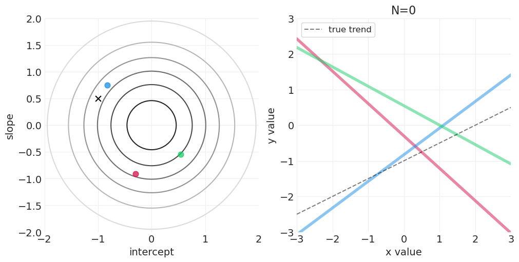
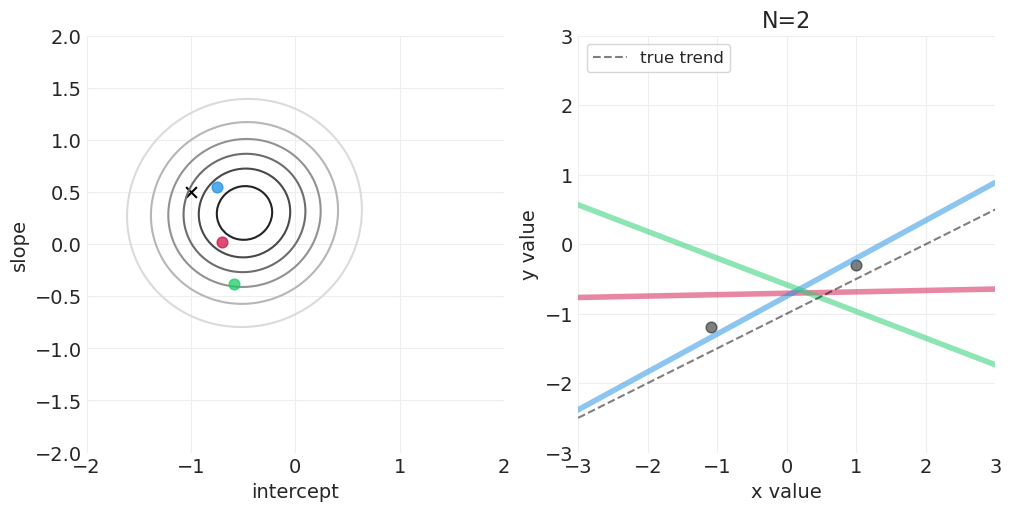
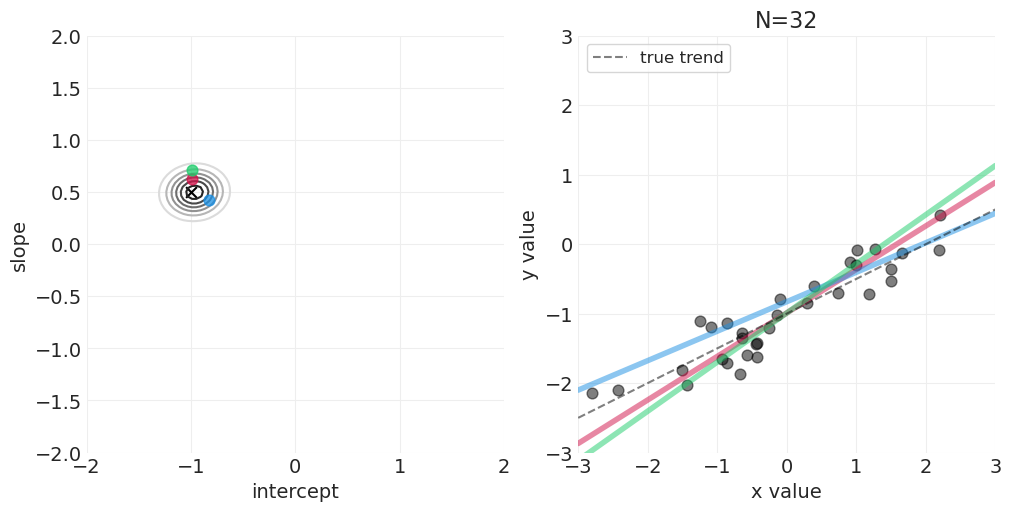
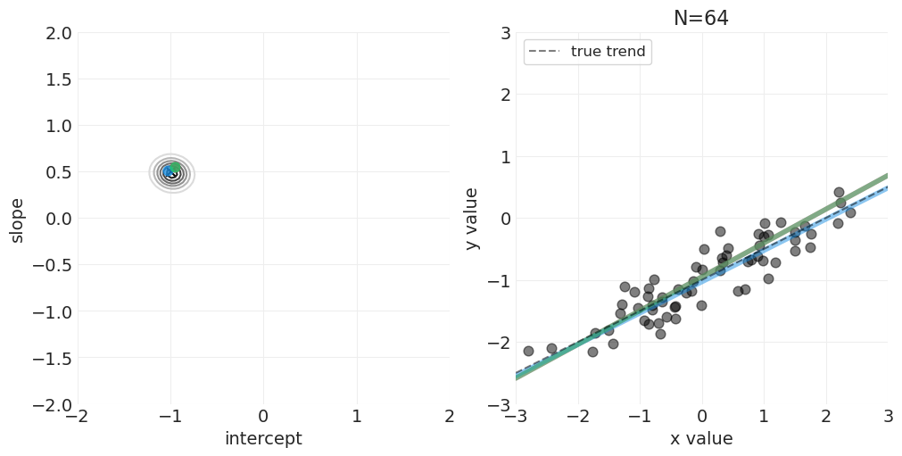
模拟后验更新#
# Generate standardized regression data for demo
np.random.seed(123)
RESOLUTION = 100
N_DATA_POINTS = 64

# Ground truth parameters
SLOPE = 0.5
INTERCEPT = -1

x = stats.norm().rvs(size=N_DATA_POINTS)
y = INTERCEPT + SLOPE * x + stats.norm.rvs(size=N_DATA_POINTS) * 0.25

slope_grid = np.linspace(-2, 2, RESOLUTION)
intercept_grid = np.linspace(-2, 2, RESOLUTION)

# Vary the sample size to show how the posterior adapts to more and more data
for n_samples in [0, 2, 4, 8, 16, 32, 64]:
    # Run the simulation
    utils.simulate_2_parameter_bayesian_learning_grid_approximation(
        x_obs=x[:n_samples],
        y_obs=y[:n_samples],
        param_a_grid=intercept_grid,
        param_b_grid=slope_grid,
        true_param_a=INTERCEPT,
        true_param_b=SLOPE,
        model_func=linear_model,
        posterior_func=linear_regression_posterior,
        param_labels=["intercept", "slope"],
        data_range_x=(-3, 3),
        data_range_y=(-3, 3),
    )
足够的网格近似—— quap vs MCMC 实现#
McElreath 在讲座的前半部分使用了二次近似——quap——这可以加速连续模型的模型拟合,这些模型的后验可以用多维正态分布来近似。但是,我们将对所有示例使用 PyMC MCMC 实现,而不会失一般性。对于讲座系列中较早使用 quap 的示例,MCMC 采样无论如何都非常快。
(4)验证模型#
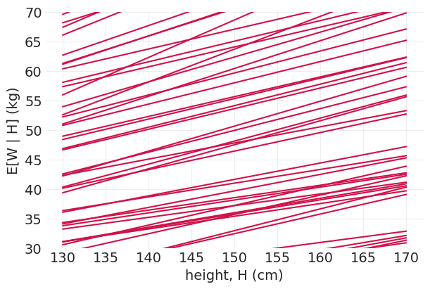
使用先验预测分布验证假设#
先验应该表达科学知识,但要柔和地表达
例如,当身高为 0 时,体重应该为 0,对吗?
体重应该(平均而言)随身高增加——即 \(\beta > 0\)
体重 (kg) 应该小于身高 (cm)
方差应该为正
关于先验的更多信息#
我们可以通过运行模拟来理解先验的影响
没有正确的先验,只有那些在科学上合理的先验
对于简单模型,先验不太重要
对于复杂模型,先验非常重要
n_simulations = 100

alphas = np.random.normal(0, 10, n_simulations)
betas = np.random.uniform(0, 1, n_simulations)  # beta should all be positive

heights = np.linspace(130, 170, 3)

fig, ax = plt.subplots(figsize=(6, 4))
for a, b in zip(alphas, betas):
    weights = a + b * heights
    plt.plot(heights, weights, color="C0")

plt.xlabel("height, H (cm)")
plt.ylabel("E[W | H] (kg)")
plt.ylim((30, 70));
基于模拟的验证和校准#
用变化的参数模拟数据
改变与模型类似的数据生成参数(例如斜率);确保估计器跟踪
确保在大样本量下,可以恢复数据生成参数
对于混杂因素/未知因素也是如此
linear_regression_inferences = []
linear_regression_models = []

sample_sizes = [1, 2, 10, 20, 50, len(H)]

for sample_size in sample_sizes:
    print(f"Sample size: {sample_size}")
    with pm.Model() as model:

        # Mutable data for posterior predictive visualization
        H_ = pm.Data("H", H[:sample_size], dims="obs_id")

        # Priors
        alpha = pm.Normal("alpha", 0, 10)  # Intercept
        beta = pm.Uniform("beta", 0, 1)  # slope
        sigma = pm.Uniform("sigma", 0, 10)  # Noise variance

        # Likelihood
        mu = alpha + beta * H_
        pm.Normal("W_obs", mu, sigma, observed=W[:sample_size], dims="obs_id")

        # Sample posterior
        inference = pm.sample(target_accept=0.99)
        linear_regression_inferences.append(inference)
        linear_regression_models.append(model)
Initializing NUTS using jitter+adapt_diag...
Sample size: 1
Multiprocess sampling (4 chains in 4 jobs)
NUTS: [alpha, beta, sigma]
Sampling 4 chains for 1_000 tune and 1_000 draw iterations (4_000 + 4_000 draws total) took 5 seconds.
There were 31 divergences after tuning. Increase `target_accept` or reparameterize.
Initializing NUTS using jitter+adapt_diag...
Sample size: 2
Multiprocess sampling (4 chains in 4 jobs)
NUTS: [alpha, beta, sigma]
Sampling 4 chains for 1_000 tune and 1_000 draw iterations (4_000 + 4_000 draws total) took 9 seconds.
There were 21 divergences after tuning. Increase `target_accept` or reparameterize.
Initializing NUTS using jitter+adapt_diag...
Sample size: 10
Multiprocess sampling (4 chains in 4 jobs)
NUTS: [alpha, beta, sigma]
Sampling 4 chains for 1_000 tune and 1_000 draw iterations (4_000 + 4_000 draws total) took 3 seconds.
Initializing NUTS using jitter+adapt_diag...
Sample size: 20
Multiprocess sampling (4 chains in 4 jobs)
NUTS: [alpha, beta, sigma]
Sampling 4 chains for 1_000 tune and 1_000 draw iterations (4_000 + 4_000 draws total) took 4 seconds.
Initializing NUTS using jitter+adapt_diag...
Sample size: 50
Multiprocess sampling (4 chains in 4 jobs)
NUTS: [alpha, beta, sigma]
Sampling 4 chains for 1_000 tune and 1_000 draw iterations (4_000 + 4_000 draws total) took 5 seconds.
Initializing NUTS using jitter+adapt_diag...
Sample size: 200
Multiprocess sampling (4 chains in 4 jobs)
NUTS: [alpha, beta, sigma]
Sampling 4 chains for 1_000 tune and 1_000 draw iterations (4_000 + 4_000 draws total) took 6 seconds.
使用后验预测分布测试模型有效性#
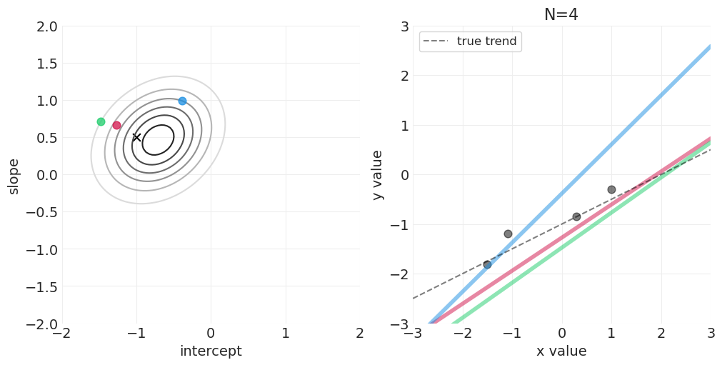
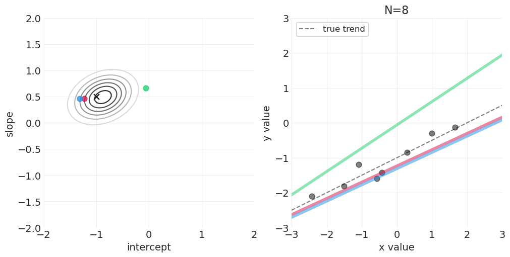
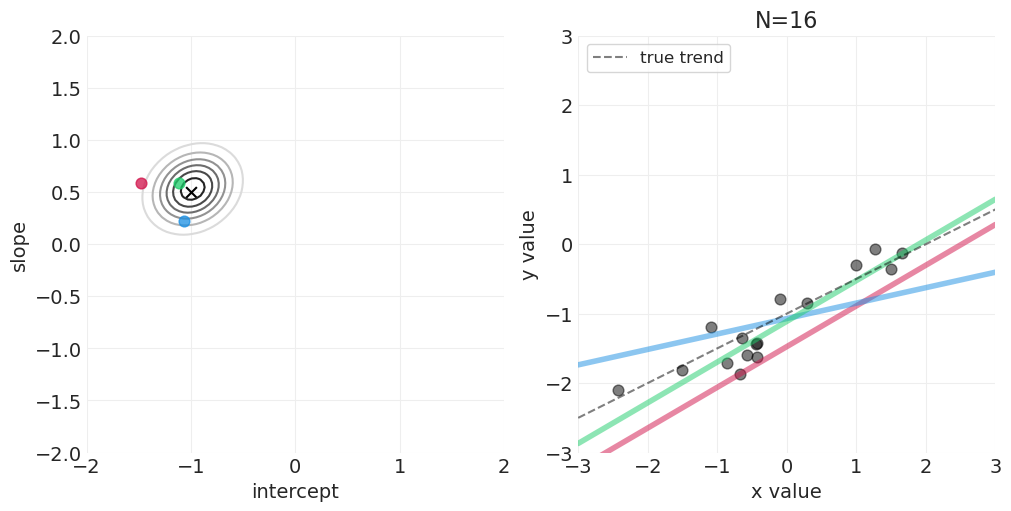
下面我们展示
后验如何随着更多观测变得更具体
后验是如何“由线组成的”——可以从后验中绘制出无限条可能的线
可以建立置信区间来传达后验拟合数据的不确定性
N_SHOW = 20
MIN_WEIGHT = 55
MAX_WEIGHT = 90


def plot_linear_regression_posterior_predictive(
    model,
    inference,
    min_height=MIN_HEIGHT,
    max_height=MAX_HEIGHT,
    min_weight=MIN_WEIGHT,
    max_weight=MAX_WEIGHT,
    N_SHOW=20,
):
    xs = np.linspace(min_height, max_height, 30)
    H_ = xr.DataArray(xs)

    # Sample Posterior Predictive with full range of heights
    with model:
        pm.set_data({"H": H_})
        ppd = pm.sample_posterior_predictive(
            inference,
            var_names=["W_obs"],
            predictions=True,
            return_inferencedata=True,
            progressbar=False,
        )

    # Plot Posterior Predictive HDI
    az.plot_hdi(H_, ppd.predictions["W_obs"], color="k", fill_kwargs=dict(alpha=0.1))

    # Plot Posterior
    posterior = inference.posterior
    lines = posterior["alpha"] + posterior["beta"] * H_
    for l in lines[0, :N_SHOW, :]:
        plt.plot(xs, l, color="k", alpha=0.5, zorder=20)

    # Formatting
    plt.xticks(np.arange(min_height, max_height + 1, 10))
    plt.xlim([min_height, max_height])
    plt.xlabel("hieght, H (cm)")

    plt.ylim([min_weight, max_weight])
    plt.yticks(np.arange(min_weight, max_weight, 10))
    plt.ylabel("weight, W (kg)")


fig, axs = plt.subplots(2, 3, figsize=(10, 8))
for ii, (sample_size, model, inference) in enumerate(
    zip(sample_sizes, linear_regression_models, linear_regression_inferences)
):
    print(f"Sample size: {sample_size}")
    plt.sca(axs[ii // 3][ii % 3])

    # Plot training data
    plt.scatter(H[:sample_size], W[:sample_size], s=80, zorder=20, alpha=0.5)
    plot_linear_regression_posterior_predictive(model, inference)
    plt.title(f"N={sample_size}")
Sampling: [W_obs]
Sampling: [W_obs]
Sample size: 1
Sample size: 2
Sampling: [W_obs]
Sampling: [W_obs]
Sample size: 10
Sample size: 20
Sampling: [W_obs]
Sampling: [W_obs]
Sample size: 50
Sample size: 200

(5)分析真实数据#
with pm.Model() as howell_model:

    # Mutable data for posterior predictive / visualization
    H_ = pm.Data("H", ADULT_HOWELL.height.values, dims="obs_ids")

    # priors
    alpha = pm.Normal("alpha", 0, 10)  # Intercept
    beta = pm.Uniform("beta", 0, 1)  # Slope
    sigma = pm.Uniform("sigma", 0, 10)  # Noise variance

    # likelihood
    mu = alpha + beta * H_
    pm.Normal("W_obs", mu, sigma, observed=ADULT_HOWELL.weight.values, dims="obs_ids")

    # Sample posterior
    howell_inference = pm.sample(target_accept=0.99)
Initializing NUTS using jitter+adapt_diag...
Multiprocess sampling (4 chains in 4 jobs)
NUTS: [alpha, beta, sigma]
Sampling 4 chains for 1_000 tune and 1_000 draw iterations (4_000 + 4_000 draws total) took 9 seconds.
az.summary(howell_inference)
| mean | sd | hdi_3% | hdi_97% | mcse_mean | mcse_sd | ess_bulk | ess_tail | r_hat | |
|---|---|---|---|---|---|---|---|---|---|
| alpha | -43.403 | 4.223 | -50.924 | -35.313 | 0.132 | 0.094 | 1011.0 | 1322.0 | 1.0 |
| beta | 0.572 | 0.027 | 0.522 | 0.623 | 0.001 | 0.001 | 1015.0 | 1256.0 | 1.0 |
| sigma | 4.284 | 0.170 | 3.944 | 4.597 | 0.005 | 0.004 | 1158.0 | 1153.0 | 1.0 |
绘制后验和参数相关性图#
from seaborn import pairplot

pairplot(
    pd.DataFrame(
        {
            "alpha": howell_inference.posterior.sel(chain=0)["alpha"],
            "beta": howell_inference.posterior.sel(chain=0)["beta"],
            "sigma": howell_inference.posterior.sel(chain=0)["sigma"],
        }
    ),
    diag_kind="kde",
    plot_kws={"alpha": 0.25},
    height=2,
);
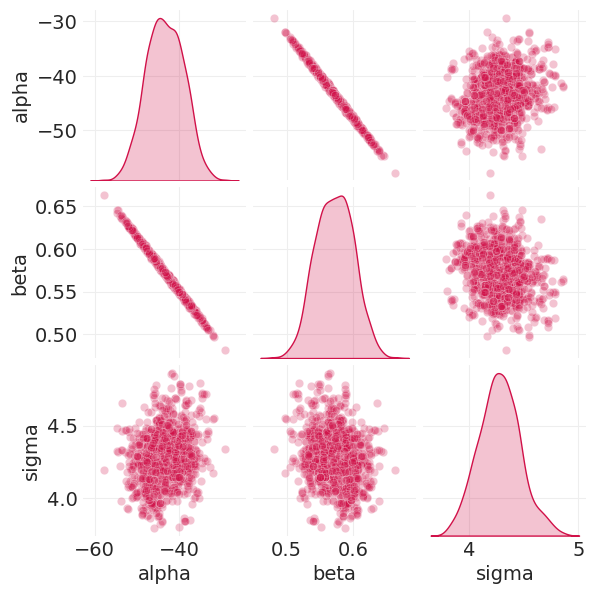
遵守定律:#
参数不是独立的
参数不能孤立地解释
相反……推出后验预测
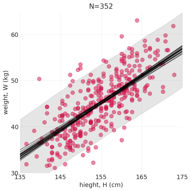
下面,我们再次展示
后验是如何“由线组成的”——可以从后验中绘制出无限条可能的线
可以建立置信区间来传达后验拟合数据的不确定性
plt.subplots(figsize=(6, 6))
plt.scatter(ADULT_HOWELL.height.values, ADULT_HOWELL.weight.values, s=80, zorder=20, alpha=0.5)
plot_linear_regression_posterior_predictive(
    howell_model, howell_inference, min_height=135, max_height=175, min_weight=30, max_weight=65
)
plt.title(f"N={len(ADULT_HOWELL)}");
Sampling: [W_obs]
许可声明#
本示例库中的所有 Notebook 均在 MIT 许可证下提供,该许可证允许修改和再分发以用于任何用途,前提是保留版权和许可证声明。
引用 PyMC 示例#
要引用此 Notebook,请使用 Zenodo 为 pymc-examples 存储库提供的 DOI。
重要提示
许多 Notebook 改编自其他来源:博客、书籍…… 在这种情况下,您也应该引用原始来源。
还请记住引用代码中使用的相关库。
这是一个 bibtex 格式的引用模板
@incollection{citekey,
  author    = "<notebook authors, see above>",
  title     = "<notebook title>",
  editor    = "PyMC Team",
  booktitle = "PyMC examples",
  doi       = "10.5281/zenodo.5654871"
}
渲染后可能如下所示