类别与曲线

此笔记本是 PyMC 移植的 Statistical Rethinking 2023 Richard McElreath 讲座系列的一部分。

视频 - 讲座 04 - 类别与曲线

# Ignore warnings
import warnings

import arviz as az
import numpy as np
import pandas as pd
import pymc as pm
import statsmodels.formula.api as smf
import utils as utils
import xarray as xr

from matplotlib import pyplot as plt
from matplotlib import style
from scipy import stats as stats

warnings.filterwarnings("ignore")

# Set matplotlib style
STYLE = "statistical-rethinking-2023.mplstyle"
style.use(STYLE)

%config InlineBackend.figure_format = 'retina'
%load_ext autoreload
%autoreload 2

线性回归 & 绘制推断

• 可用于近似大多数事物，甚至是非线性现象（例如 GLM）

• 我们需要将因果思考融入到…

  • …我们如何构建统计模型

  • …我们如何处理和解释结果

类别

• 非连续性原因

• 离散、无序的类型

• 按类别分层：为每个类别拟合单独的回归（例如直线）

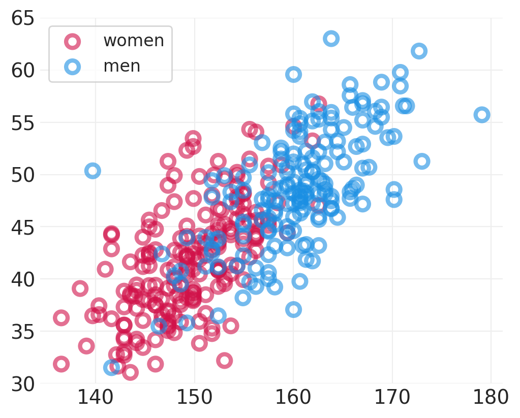
重访 Howell 数据集

HOWELL = utils.load_data("Howell1")

# Adult data
ADULT_HOWELL = HOWELL[HOWELL.age >= 18]

# Split by the Sex Category
SEX = ["women", "men"]

plt.subplots(figsize=(5, 4))
for ii, label in enumerate(SEX):
    utils.plot_scatter(
        ADULT_HOWELL[ADULT_HOWELL.male == ii].height,
        ADULT_HOWELL[ADULT_HOWELL.male == ii].weight,
        color=f"C{ii}",
        label=label,
    )
plt.ylim([30, 65])
plt.legend();

# Draw the mediation graph
utils.draw_causal_graph(edge_list=[("H", "W"), ("S", "H"), ("S", "W")], graph_direction="LR")

首先进行科学思考

• 身高、体重和性别是如何 因果 相关的？

• 身高、体重和性别是如何 统计 相关的？

原因不在数据中

身高应该影响体重，反之亦然

• ✅ \(H \rightarrow W\)

• ❌ \(H \leftarrow W\)

性别应该影响身高，反之亦然

• ❌ \(H \rightarrow S\)

• ✅ \(H \leftarrow S\)

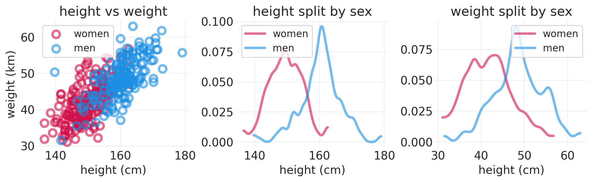
# Split height by the Sex Category


def plot_height_weight_distributions(data):
    fig, axs = plt.subplots(1, 3, figsize=(10, 3))
    plt.sca(axs[0])

    for ii, label in enumerate(SEX):
        utils.plot_scatter(
            data[data.male == ii].height,
            data[data.male == ii].weight,
            color=f"C{ii}",
            label=label,
        )
    plt.xlabel("height (cm)")
    plt.ylabel("weight (km)")
    plt.legend()
    plt.title("height vs weight")

    for vv, var in enumerate(["height", "weight"]):
        plt.sca(axs[vv + 1])
        for ii in range(2):
            az.plot_dist(
                data.loc[data.male == ii, var].values,
                color=f"C{ii}",
                label=SEX[ii],
                bw=1,
                plot_kwargs=dict(linewidth=3, alpha=0.6),
            )
        plt.title(f"{var} split by sex")
        plt.xlabel("height (cm)")
        plt.legend()


plot_height_weight_distributions(ADULT_HOWELL)

因果图定义了一组函数关系

\[\begin{split} \begin{align*} H &= f_H(S) \\ W &= f_W(H, S) \end{align*} \end{split}\]

还可以包括对 \(S\) 的不可观察的因果影响 \(T\) (见下图)

\[\begin{split} \begin{align*} H &= f_H(S, U) \\ W &= f_W(H, S, V) \\ S &= f_S(T) \end{align*} \end{split}\]

注意：我们使用 \(T\) 作为未观察到的变量，而不是 \(W\) 以避免在讲座中重复。

utils.draw_causal_graph(
    edge_list=[("H", "W"), ("S", "H"), ("S", "W"), ("V", "W"), ("U", "H"), ("T", "S")],
    node_props={
        "T": {"style": "dashed"},
        "U": {"style": "dashed"},
        "V": {"style": "dashed"},
        "unobserved": {"style": "dashed"},
    },
    graph_direction="LR",
)

合成人

utils.draw_causal_graph(
    edge_list=[("H", "W"), ("S", "H"), ("S", "W"), ("V", "W"), ("U", "H"), ("T", "S")],
    node_props={
        "T": {"style": "dashed", "color": "lightgray"},
        "U": {"style": "dashed", "color": "lightgray"},
        "V": {"style": "dashed", "color": "lightgray"},
        "unobserved": {"style": "dashed", "color": "lightgray"},
    },
    edge_props={
        ("T", "S"): {"color": "lightgray"},
        ("U", "H"): {"color": "lightgray"},
        ("V", "W"): {"color": "lightgray"},
    },
    graph_direction="LR",
)

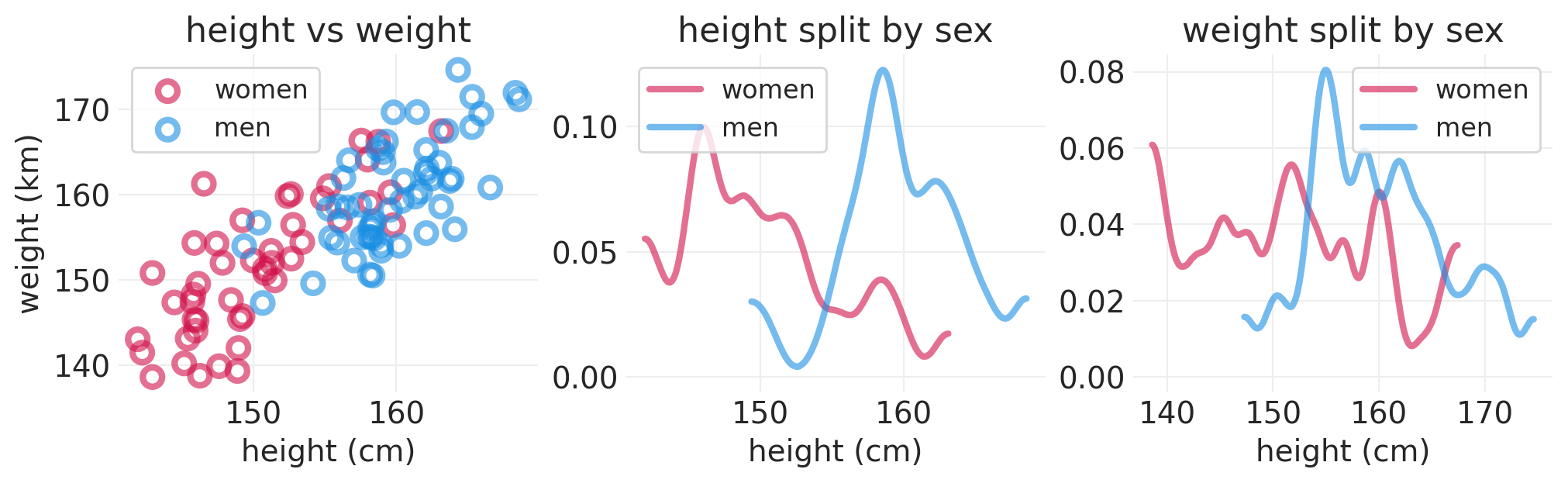
def simulate_sex_height_weight(
    S: np.ndarray,
    beta: np.ndarray = np.array([1, 1]),
    alpha: np.ndarray = np.array([0, 0]),
    female_mean_height: float = 150,
    male_mean_height: float = 160,
) -> np.ndarray:
    """
    Generative model for the effect of Sex on height & weight

    S: np.array[int]
        The 0/1 indicator variable sex. 1 means 'male'
    beta: np.array[float]
        Lenght 2 slope coefficient for each sex
    alpha: np.array[float]
        Length 2 intercept for each sex
    """
    N = len(S)
    H = np.where(S, male_mean_height, female_mean_height) + stats.norm(0, 5).rvs(size=N)
    W = alpha[S] + beta[S] * H + stats.norm(0, 5).rvs(size=N)

    return pd.DataFrame({"height": H, "weight": W, "male": S})


synthetic_sex = stats.bernoulli(p=0.5).rvs(size=100).astype(int)
synthetic_people = simulate_sex_height_weight(S=synthetic_sex)
plot_height_weight_distributions(synthetic_people)
synthetic_people.head()

	身高	体重	男性
0	150.367120	156.692279	1
1	142.944365	138.574022	0
2	161.321188	159.747881	1
3	159.279357	166.230071	1
4	146.539279	161.260587	0

首先进行科学思考

不同的因果问题需要不同的统计模型

• 问题 1：\(H\) 对 \(W\) 的因果效应是什么？

• 问题 2：\(S\) 对 \(W\) 的 总 因果效应是什么？

• 问题 3：\(S\) 对 \(W\) 的 直接 因果效应是什么？

回答最后两个问题需要不同的统计模型，但这都需要按 \(S\) 分层

从估计量到估计值

\(H\) 对 \(W\) 的因果效应 (Q1)

utils.draw_causal_graph(
    edge_list=[("H", "W"), ("S", "W"), ("S", "H")],
    node_props={"H": {"color": "red"}, "W": {"color": "red"}},
    edge_props={
        ("H", "W"): {"color": "red"},
    },
    graph_direction="LR",
)

\(S\) 对 \(W\) 的 总 因果效应 (Q2)

utils.draw_causal_graph(
    edge_list=[("H", "W"), ("S", "W"), ("S", "H")],
    node_props={"S": {"color": "red"}, "W": {"color": "red"}},
    edge_props={
        ("S", "H"): {"color": "red"},
        ("H", "W"): {"color": "red"},
        ("S", "W"): {"color": "red"},
    },
    graph_direction="LR",
)

\(S\) 对 \(W\) 的 直接 因果效应 (Q3)

utils.draw_causal_graph(
    edge_list=[("H", "W"), ("S", "W"), ("S", "H")],
    node_props={"S": {"color": "red"}, "W": {"color": "red"}},
    edge_props={("S", "W"): {"color": "red"}},
    graph_direction="LR",
)

按 S 分层：为 \(S\) 可以取的每个值恢复不同的估计值

绘制因果猫头鹰 🦉

通过 指示变量 实现类别

• 通用代码：可以扩展到任意数量的类别

• 更适合先验规范

• 有助于多层模型规范

对于类别 \(C = [C_1, C_2, ... C_D]\)

\[\begin{split} \begin{align*} \alpha &= [\alpha_1, \alpha_2, ... \alpha_D] \\ y_i &\sim \text{Normal}(\mu_i, \sigma) \\ \mu_i &= \alpha_{C[i]} \end{align*} \end{split}\]

对于性别 \(S\in \{M, F\}\)，我们可以将性别特定的体重 \(W\) 建模为

\[\begin{split} \begin{align*} W_i &\sim \text{Normal}(\mu_i, \sigma) \\ \mu_i &= \alpha_{S[i]} \\ \alpha &= [\alpha_F, \alpha_M] \\ \alpha_j &\sim \text{Normal}(60, 10) \\ \sigma &\sim \text{Uniform}(0, 10) \end{align*} \end{split}\]

测试

性别对体重的总因果效应

utils.draw_causal_graph(
    edge_list=[("H", "W"), ("S", "W"), ("S", "H")],
    node_props={"S": {"color": "blue"}, "W": {"color": "red"}, "stratified": {"color": "blue"}},
    edge_props={
        ("S", "H"): {"color": "red"},
        ("H", "W"): {"color": "red"},
        ("S", "W"): {"color": "red"},
    },
    graph_direction="LR",
)

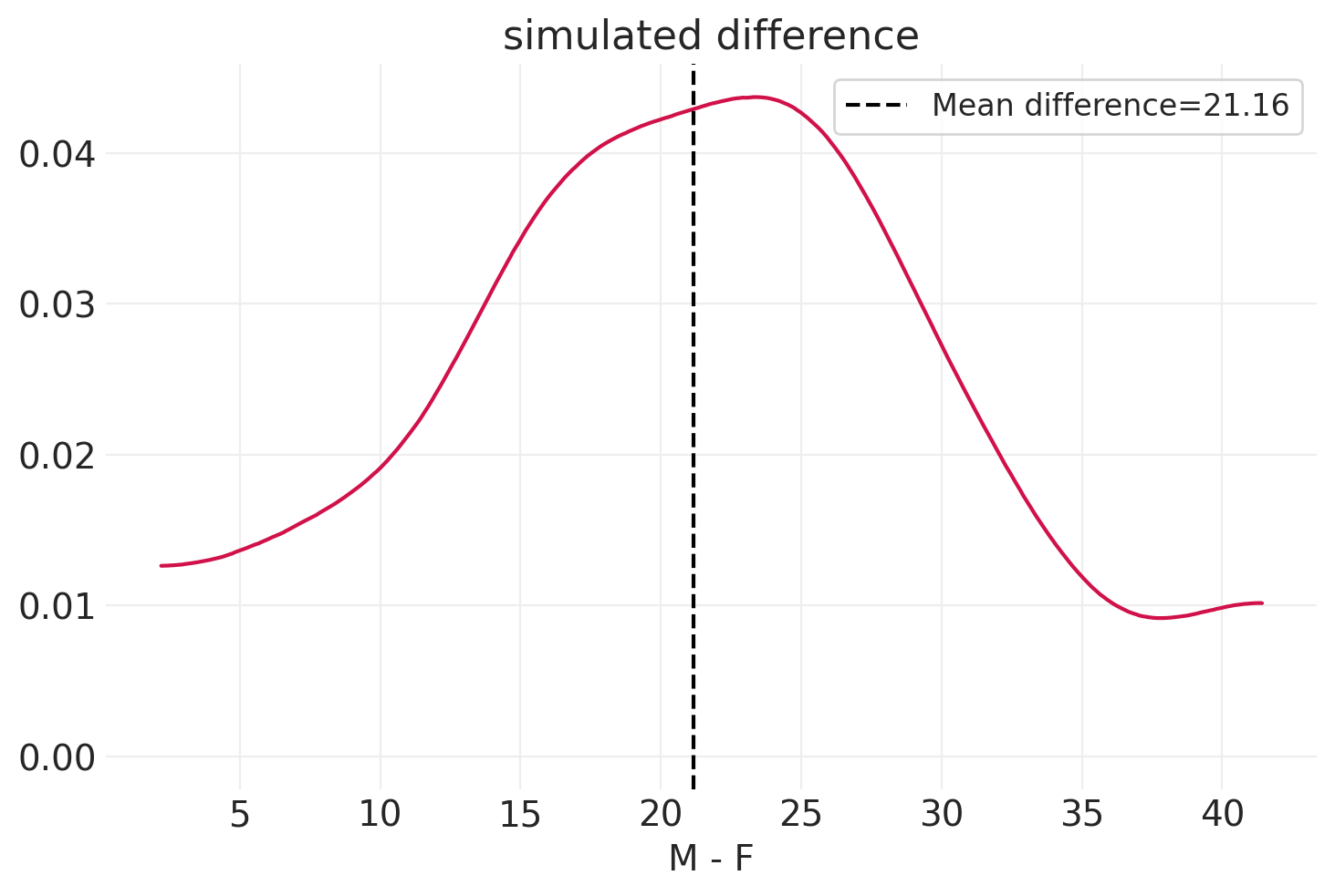
np.random.seed(12345)
n_simulations = 100
simulated_females = simulate_sex_height_weight(
    S=np.zeros(n_simulations).astype(int), beta=np.array((0.5, 0.6))
)

simulated_males = simulate_sex_height_weight(
    S=np.ones(n_simulations).astype(int), beta=np.array((0.5, 0.6))
)

simulated_delta = simulated_males - simulated_females
mean_simualted_delta = simulated_delta.mean()
az.plot_dist(simulated_delta["weight"].values)
plt.axvline(
    mean_simualted_delta["weight"],
    linestyle="--",
    color="k",
    label="Mean difference" + f"={mean_simualted_delta['weight']:1.2f}",
)
plt.xlabel("M - F")
plt.legend()
plt.title("simulated difference");

拟合合成样本的总效应

按 \(S\) 分层

def fit_total_effect_model(data):

    SEX_ID, SEX = pd.factorize(["M" if s else "F" for s in data["male"].values])

    with pm.Model(coords={"SEX": SEX}) as model:
        # Data
        S = pm.Data("S", SEX_ID)

        # Priors
        sigma = pm.Uniform("sigma", 0, 10)
        alpha = pm.Normal("alpha", 60, 10, dims="SEX")

        # Likelihood
        mu = alpha[S]
        pm.Normal("W_obs", mu, sigma, observed=data["weight"])

        inference = pm.sample()

    return inference, model


# Concatentate simulations and code sex
simulated_people = pd.concat([simulated_females, simulated_males])
simulated_total_effect_inference, simulated_total_effect_model = fit_total_effect_model(
    simulated_people
)

Initializing NUTS using jitter+adapt_diag...
Multiprocess sampling (4 chains in 4 jobs)
NUTS: [sigma, alpha]

Sampling 4 chains for 1_000 tune and 1_000 draw iterations (4_000 + 4_000 draws total) took 1 seconds.

simulated_summary = az.summary(simulated_total_effect_inference, var_names=["alpha", "sigma"])
simulated_delta = (simulated_summary.iloc[1] - simulated_summary.iloc[0])["mean"]
print(f"Delta in average sex-specific weight: {simulated_delta:1.2f}")

simulated_summary

Delta in average sex-specific weight: 21.09

	均值	标准差	hdi_3%	hdi_97%	mcse_mean	mcse_sd	ess_bulk	ess_tail	r_hat
alpha[F]	74.860	0.589	73.735	75.948	0.008	0.006	4919.0	2724.0	1.0
alpha[M]	95.947	0.597	94.784	97.039	0.008	0.006	5017.0	2742.0	1.0
sigma	5.919	0.295	5.388	6.489	0.004	0.003	6300.0	3087.0	1.0

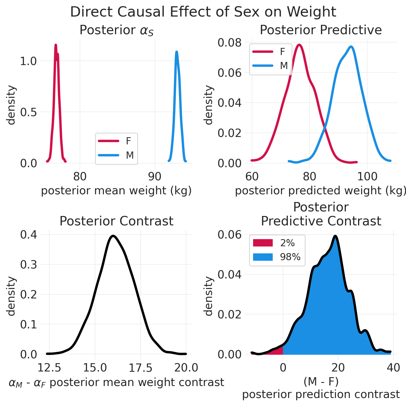
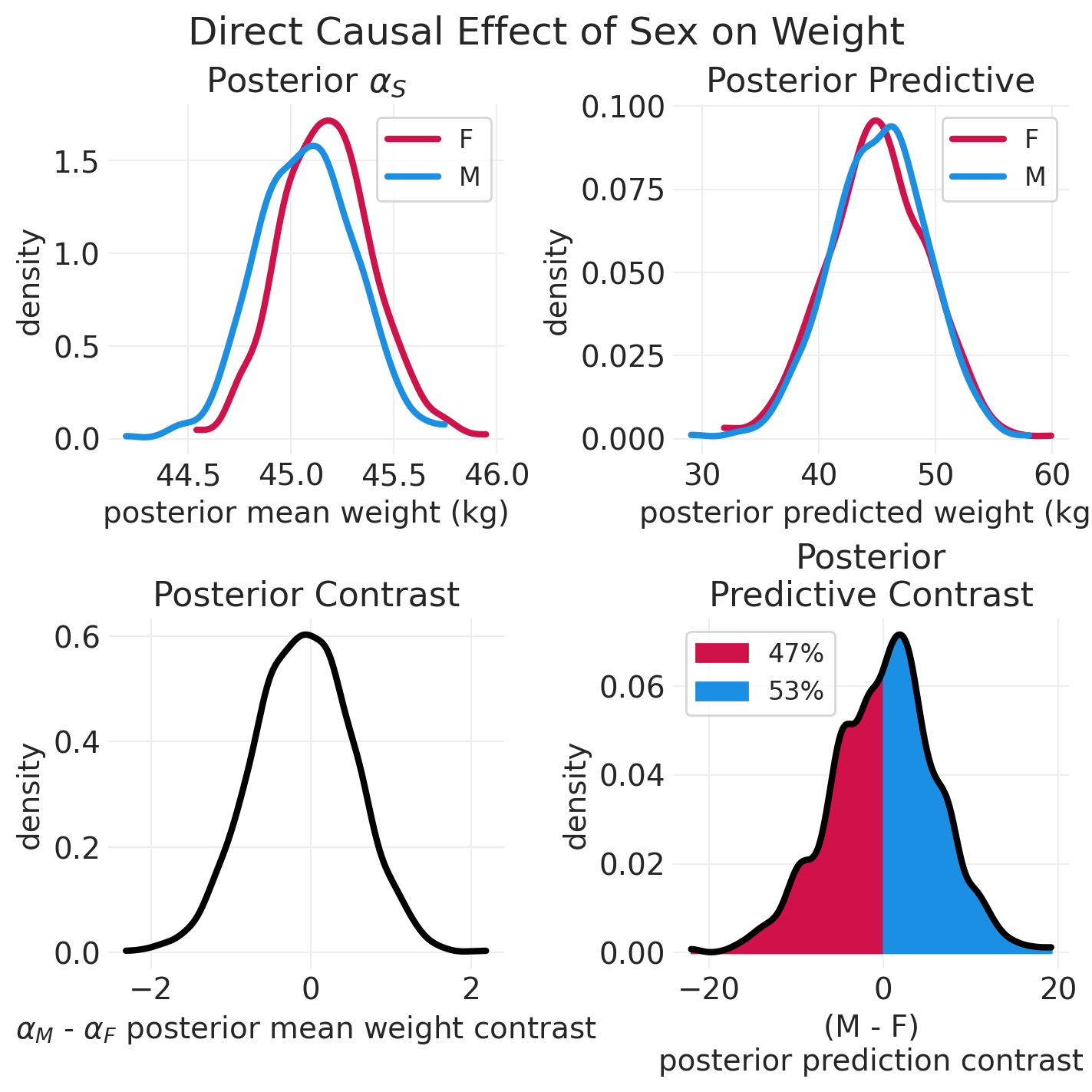
# Plotting helper functions


def plot_model_posterior(inference, effect_type: str = "Total"):
    np.random.seed(123)
    sex = ["F", "M"]
    posterior = inference.posterior

    fig, axs = plt.subplots(2, 2, figsize=(7, 7))

    # Posterior mean
    plt.sca(axs[0][0])
    for ii, s in enumerate(sex):
        posterior_mean = posterior["alpha"].sel(SEX=s).mean(dim="chain")
        az.plot_dist(posterior_mean, color=f"C{ii}", label=s, plot_kwargs=dict(linewidth=3))

    plt.xlabel("posterior mean weight (kg)")
    plt.ylabel("density")
    plt.legend()
    plt.title("Posterior $\\alpha_S$")

    # Posterior Predictive
    plt.sca(axs[0][1])
    posterior_prediction_std = posterior["sigma"].mean(dim=["chain"])
    posterior_prediction = {}

    for ii, s in enumerate(sex):
        posterior_prediction_mean = posterior.sel(SEX=s)["alpha"].mean(dim=["chain"])
        posterior_prediction[s] = stats.norm.rvs(
            posterior_prediction_mean, posterior_prediction_std
        )
        az.plot_dist(
            posterior_prediction[s], color=f"C{ii}", label=s, plot_kwargs=dict(linewidth=3)
        )

    plt.xlabel("posterior predicted weight (kg)")
    plt.ylabel("density")
    plt.legend()
    plt.title("Posterior Predictive")

    # Plost Contrasts
    ## Posterior Contrast
    plt.sca(axs[1][0])
    posterior_contrast = posterior.sel(SEX="M")["alpha"] - posterior.sel(SEX="F")["alpha"]
    az.plot_dist(posterior_contrast, color="k", plot_kwargs=dict(linewidth=3))
    plt.xlabel("$\\alpha_M$ - $\\alpha_F$ posterior mean weight contrast")
    plt.ylabel("density")
    plt.title("Posterior Contrast")

    ## Posterior Predictive Contrast
    plt.sca(axs[1][1])
    posterior_predictive_contrast = posterior_prediction["M"] - posterior_prediction["F"]
    n_draws = len(posterior_predictive_contrast)
    kde_ax = az.plot_dist(
        posterior_predictive_contrast, color="k", bw=1, plot_kwargs=dict(linewidth=3)
    )

    # Shade underneath posterior predictive contrast
    kde_x, kde_y = kde_ax.get_lines()[0].get_data()

    # Proportion of PPD contrast below zero
    neg_idx = kde_x < 0
    neg_prob = 100 * np.sum(posterior_predictive_contrast < 0) / n_draws
    plt.fill_between(
        x=kde_x[neg_idx],
        y1=np.zeros(sum(neg_idx)),
        y2=kde_y[neg_idx],
        color="C0",
        label=f"{neg_prob:1.0f}%",
    )

    # Proportion of PPD contrast above zero (inclusive)
    pos_idx = kde_x >= 0
    pos_prob = 100 * np.sum(posterior_predictive_contrast >= 0) / n_draws
    plt.fill_between(
        x=kde_x[pos_idx],
        y1=np.zeros(sum(pos_idx)),
        y2=kde_y[pos_idx],
        color="C1",
        label=f"{pos_prob:1.0f}%",
    )

    plt.xlabel("(M - F)\nposterior prediction contrast")
    plt.ylabel("density")
    plt.legend()
    plt.title("Posterior\nPredictive Contrast")
    plt.suptitle(f"{effect_type} Causal Effect of Sex on Weight", fontsize=18)


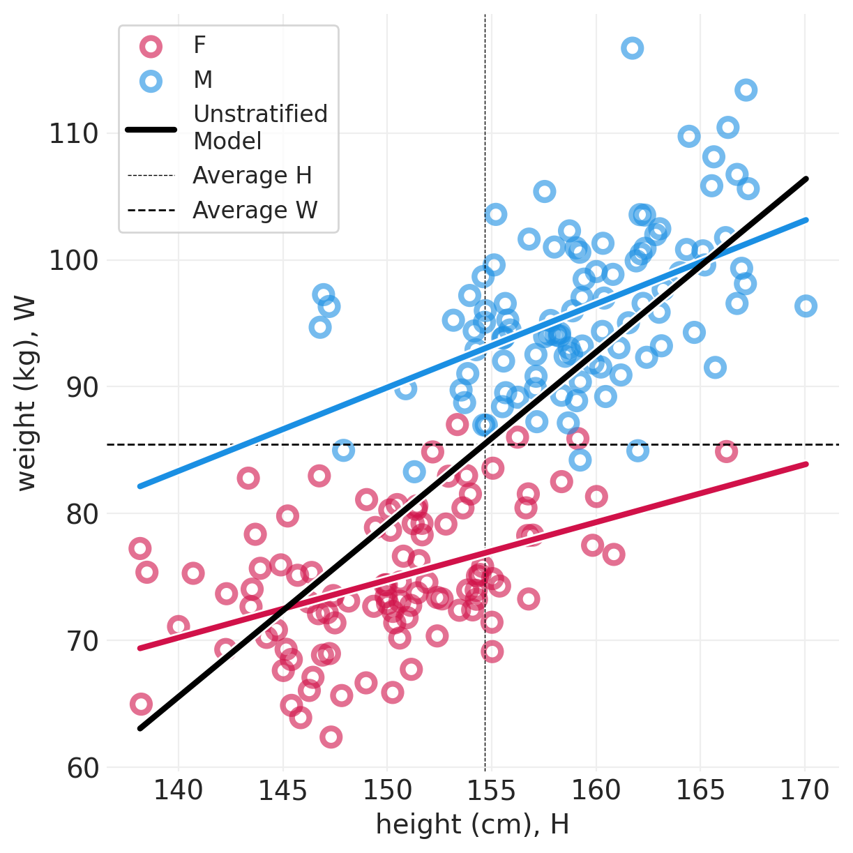
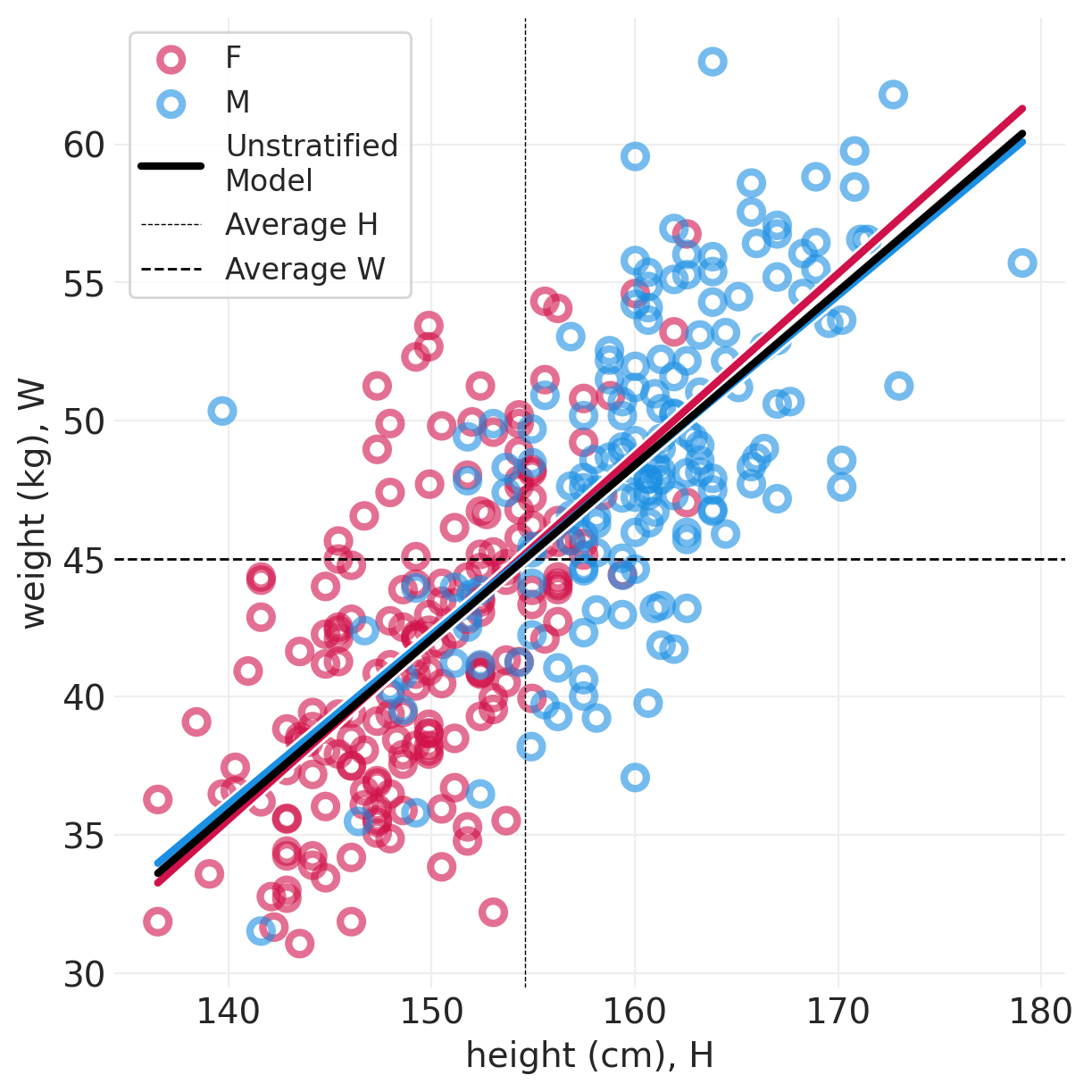
def plot_posterior_lines(data, inference, centered=False):
    plt.subplots(figsize=(6, 6))

    min_height = data.height.min()
    max_height = data.height.max()
    xs = np.linspace(min_height, max_height, 10)
    for ii, s in enumerate(["F", "M"]):
        sex_idx = data.male == ii
        utils.plot_scatter(
            xs=data[sex_idx].height, ys=data[sex_idx].weight, color=f"C{ii}", label=s
        )

        posterior_mean = inference.posterior.sel(SEX=s).mean(dim=("chain", "draw"))
        posterior_mean_alpha = posterior_mean["alpha"].values
        posterior_mean_beta = getattr(posterior_mean, "beta", pd.Series([0])).values

        if centered:
            pred_x = xs - data.height.mean()
        else:
            pred_x = xs

        ys = posterior_mean_alpha + posterior_mean_beta * pred_x
        utils.plot_line(xs, ys, label=None, color=f"C{ii}")

    # Model fit to both sexes simultaneously
    global_model = smf.ols("weight ~ height", data=data).fit()
    ys = global_model.params.Intercept + global_model.params.height * xs
    utils.plot_line(xs, ys, color="k", label="Unstratified\nModel")

    plt.axvline(
        data["height"].mean(), label="Average H", linewidth=0.5, linestyle="--", color="black"
    )
    plt.axhline(
        data["weight"].mean(), label="Average W", linewidth=1, linestyle="--", color="black"
    )
    plt.legend()
    plt.xlabel("height (cm), H")
    plt.ylabel("weight (kg), W");

plot_posterior_lines(simulated_people, simulated_total_effect_inference, centered=True)

plot_model_posterior(simulated_total_effect_inference)

分析真实样本

adult_howell_total_effect_inference, adult_howell_total_effect_model = fit_total_effect_model(
    ADULT_HOWELL
)

Initializing NUTS using jitter+adapt_diag...
Multiprocess sampling (4 chains in 4 jobs)
NUTS: [sigma, alpha]

Sampling 4 chains for 1_000 tune and 1_000 draw iterations (4_000 + 4_000 draws total) took 1 seconds.

adult_howell_total_effect_summary = az.summary(
    adult_howell_total_effect_inference, var_names=["alpha"]
)
adult_howell_total_effect_delta = (
    adult_howell_total_effect_summary.iloc[1] - adult_howell_total_effect_summary.iloc[0]
)["mean"]
print(f"Delta in average sex-specific weight: {adult_howell_total_effect_delta:1.2f}")

adult_howell_summary = az.summary(adult_howell_total_effect_inference)
adult_howell_summary

Delta in average sex-specific weight: -6.77

	均值	标准差	hdi_3%	hdi_97%	mcse_mean	mcse_sd	ess_bulk	ess_tail	r_hat
alpha[M]	48.617	0.427	47.835	49.428	0.005	0.004	6184.0	3360.0	1.0
alpha[F]	41.848	0.397	41.100	42.581	0.005	0.004	5639.0	2990.0	1.0
sigma	5.523	0.206	5.149	5.922	0.003	0.002	5560.0	3137.0	1.0

始终进行对比

• 需要比较类别之间的 对比

• 永远无效地计算 分布的重叠

  • 这意味着 不比较 p 值的置信区间

• 计算分布的差异 – 对比分布

plot_model_posterior(adult_howell_total_effect_inference)

plot_posterior_lines(ADULT_HOWELL, adult_howell_total_effect_inference, True)

\(S\) 对 \(W\) 的 直接 因果效应？

我们需要另一个模型/估计量来估计这个量。我们按 \(S\) 和 \(H\) 分层；按 \(H\) 分层以阻止 \(S\) 通过 \(H\) 的路径

utils.draw_causal_graph(
    edge_list=[("H", "W"), ("S", "W"), ("S", "H")],
    node_props={
        "S": {"color": "blue"},
        "W": {"color": "red"},
        "H": {"color": "blue"},
        "stratified": {"color": "blue"},
    },
    edge_props={("S", "W"): {"color": "red"}},
    graph_direction="LR",
)

\[\begin{split} \begin{align*} W_i &\sim \text{Normal}(\mu_i, \sigma) \\ \mu_i &= \alpha_{S[i]} + \beta_{S[i]} (H_i - \bar H) \end{align*} \end{split}\]

我们已经在其中 中心化了身高，这意味着

• \(\beta\) 缩放 \(H_i\) 与平均身高的差异

• \(\alpha\) 是一个人身高为平均身高时的体重

• 全局模型拟合到所有数据位于全局平均身高和体重的交点

模拟更多人

ALPHA = 0.9
np.random.seed(1234)
n_synthetic_people = 200

synthetic_sex = stats.bernoulli.rvs(p=0.5, size=n_synthetic_people)
synthetic_people = simulate_sex_height_weight(
    S=synthetic_sex,
    beta=np.array([0.5, 0.5]),  # Same relationship between height & weight
    alpha=np.array([0.0, 10]),  # 10kg "boost for Males"
)

分析合成人

def fit_direct_effect_weight_model(data):

    SEX_ID, SEX = pd.factorize(["M" if s else "F" for s in data["male"].values])

    with pm.Model(coords={"SEX": SEX}) as model:
        # Data
        S = pm.Data("S", SEX_ID, dims="obs_ids")
        H = pm.Data("H", data["height"].values, dims="obs_ids")
        Hbar = pm.Data("Hbar", data["height"].mean())

        # Priors
        sigma = pm.Uniform("sigma", 0, 10)
        alpha = pm.Normal("alpha", 60, 10, dims="SEX")
        beta = pm.Uniform("beta", 0, 1, dims="SEX")  # postive slopes only

        # Likelihood
        mu = alpha[S] + beta[S] * (H - Hbar)
        pm.Normal("W_obs", mu, sigma, observed=data["weight"].values, dims="obs_ids")

        inference = pm.sample()

    return inference, model

direct_effect_simulated_inference, direct_effect_simulated_model = fit_direct_effect_weight_model(
    simulated_people
)

Initializing NUTS using jitter+adapt_diag...
Multiprocess sampling (4 chains in 4 jobs)
NUTS: [sigma, alpha, beta]

Sampling 4 chains for 1_000 tune and 1_000 draw iterations (4_000 + 4_000 draws total) took 1 seconds.

plot_posterior_lines(simulated_people, direct_effect_simulated_inference, centered=True)

• 间接效应：男性和女性具有特定的斜率 - 在此模拟中，它们是相同的斜率，因此是平行线

• 直接效应：无论斜率如何，都会有一个 delta。– 在此模拟中，\(S\)=M 始终重 10 公斤，因此蓝色始终高于红色

plot_model_posterior(direct_effect_simulated_inference, "Direct")

分析真实样本

direct_effect_howell_inference, direct_effect_howell_model = fit_direct_effect_weight_model(
    ADULT_HOWELL
)

Initializing NUTS using jitter+adapt_diag...
Multiprocess sampling (4 chains in 4 jobs)
NUTS: [sigma, alpha, beta]

Sampling 4 chains for 1_000 tune and 1_000 draw iterations (4_000 + 4_000 draws total) took 1 seconds.

plot_posterior_lines(ADULT_HOWELL, direct_effect_howell_inference, True)

对比

plot_model_posterior(direct_effect_howell_inference, "Direct")

每个高度的对比

def plot_heightwise_contrast(model, inference):
    heights = np.linspace(130, 190, 100)
    ppds = {}
    for ii, s in enumerate(["F", "M"]):
        with model:
            pm.set_data(
                {"S": np.ones_like(heights).astype(int) * ii, "H": heights, "Hbar": heights.mean()}
            )
            ppds[s] = pm.sample_posterior_predictive(
                inference, extend_inferencedata=False
            ).posterior_predictive["W_obs"]

    ppd_contrast = ppds["M"] - ppds["F"]

    # Plot contours
    for prob in [0.5, 0.75, 0.95, 0.99]:
        az.plot_hdi(heights, ppd_contrast, hdi_prob=prob, color="gray")

    plt.axhline(0, linestyle="--", color="k")
    plt.xlabel("height, H (cm)")
    plt.ylabel("weight W contrast (M-F)")
    plt.xlim([130, 190])

plot_heightwise_contrast(direct_effect_howell_model, direct_effect_howell_inference)

Sampling: [W_obs]

Sampling: [W_obs]

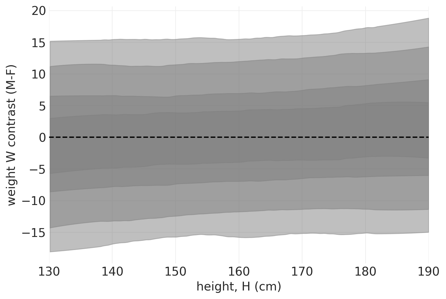
当按身高分层时，我们看到性别对身高几乎没有因果效应。即 对体重的因果效应的绝大部分是通过身高实现的。

# Try on the simulated data
plot_heightwise_contrast(direct_effect_simulated_model, direct_effect_simulated_inference)

Sampling: [W_obs]

Sampling: [W_obs]

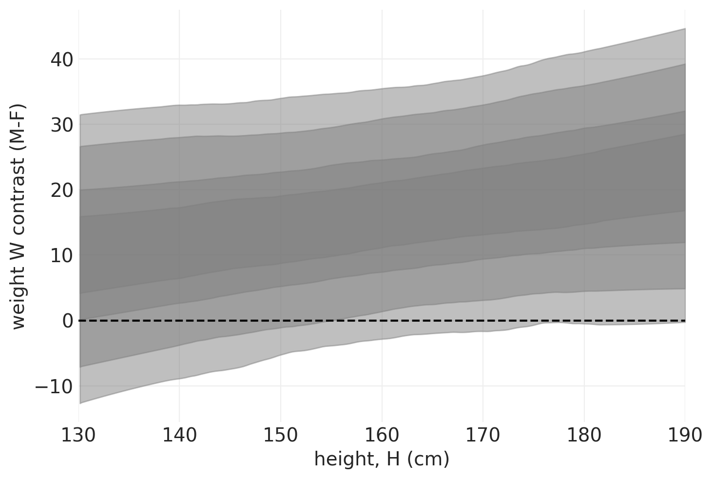
我们可以看到，在模拟数据中，男性始终比女性重，这与模拟结果一致

从直线到曲线

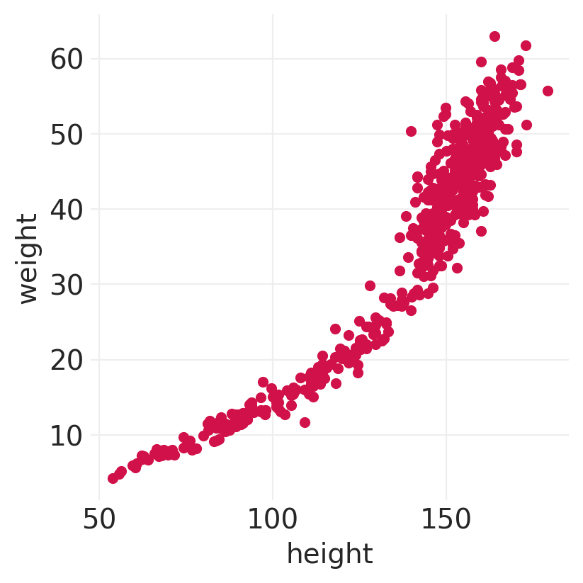
并非所有关系都是线性的

• 例如，在 Howell 数据集中，我们可以看到，如果我们包括所有年龄段，身高和体重之间的关系是非线性的

• 线性模型可以拟合曲线

• 仍然不是机械模型

fig, ax = plt.subplots(figsize=(4, 4))
HOWELL.plot(x="height", y="weight", kind="scatter", ax=ax);

多项式线性模型

\[\mu_i = \alpha + \sum_i^D \beta_i x^D \]

多项式模型的问题

• 对称 – 奇怪的边缘异常

• 全局模型，因此没有局部插值

• 容易通过增加项数过度拟合

二次多项式模型

\[\mu_i = \alpha + \beta_2 x + \beta_2 x^2 \]

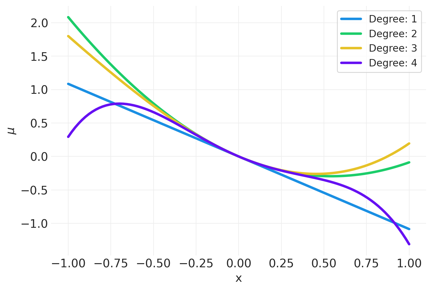
def plot_polynomial_sample(degree, random_seed=123):
    np.random.seed(random_seed)
    xs = np.linspace(-1, 1, 100)
    ys = 0
    for d in range(1, degree + 1):
        beta_d = np.random.randn()
        ys += beta_d * xs**d

    utils.plot_line(xs, ys, color=f"C{degree}", label=f"Degree: {degree}")
    plt.legend()
    plt.xlabel("x")
    plt.ylabel("$\\mu$")


for degree in [1, 2, 3, 4]:
    plot_polynomial_sample(degree)

模拟二次多项式模型的贝叶斯更新

对于以下模拟，我们将使用自定义实用程序函数 utils.simulate_2_parameter_bayesian_learning_grid_approximation 来模拟通用贝叶斯后验更新模拟。这是该函数的 API（有关更多详细信息，请参见 utils.py）

help(utils.simulate_2_parameter_bayesian_learning_grid_approximation)

Help on function simulate_2_parameter_bayesian_learning_grid_approximation in module utils:

simulate_2_parameter_bayesian_learning_grid_approximation(x_obs, y_obs, param_a_grid, param_b_grid, true_param_a, true_param_b, model_func, posterior_func, n_posterior_samples=3, param_labels=None, data_range_x=None, data_range_y=None)
    General function for simulating Bayesian learning in a 2-parameter model
    using grid approximation.

    Parameters
    ----------
    x_obs : np.ndarray
        The observed x values
    y_obs : np.ndarray
        The observed y values
    param_a_grid: np.ndarray
        The range of values the first model parameter in the model can take.
        Note: should have same length as param_b_grid.
    param_b_grid: np.ndarray
        The range of values the second model parameter in the model can take.
        Note: should have same length as param_a_grid.
    true_param_a: float
        The true value of the first model parameter, used for visualizing ground
        truth
    true_param_b: float
        The true value of the second model parameter, used for visualizing ground
        truth
    model_func: Callable
        A function `f` of the form `f(x, param_a, param_b)`. Evaluates the model
        given at data points x, given the current state of parameters, `param_a`
        and `param_b`. Returns a scalar output for the `y` associated with input
        `x`.
    posterior_func: Callable
        A function `f` of the form `f(x_obs, y_obs, param_grid_a, param_grid_b)
        that returns the posterior probability given the observed data and the
        range of parameters defined by `param_grid_a` and `param_grid_b`.
    n_posterior_samples: int
        The number of model functions sampled from the 2D posterior
    param_labels: Optional[list[str, str]]
        For visualization, the names of `param_a` and `param_b`, respectively
    data_range_x: Optional len-2 float sequence
        For visualization, the upper and lower bounds of the domain used for model
        evaluation
    data_range_y: Optional len-2 float sequence
        For visualization, the upper and lower bounds of the range used for model
        evaluation.

贝叶斯学习模拟所需的函数

def quadratic_polynomial_model(x, beta_1, beta_2):
    return beta_1 * x + beta_2 * x**2


def quadratic_polynomial_regression_posterior(
    x_obs, y_obs, beta_1_grid, beta_2_grid, likelihood_prior_std=1.0
):

    beta_1_grid = beta_1_grid.ravel()
    beta_2_grid = beta_2_grid.ravel()

    log_prior_beta_1 = stats.norm(0, 1).logpdf(beta_1_grid)
    log_prior_beta_2 = stats.norm(0, 1).logpdf(beta_2_grid)

    log_likelihood = np.array(
        [
            stats.norm(b1 * x_obs + b2 * x_obs**2, likelihood_prior_std).logpdf(y_obs)
            for b1, b2 in zip(beta_1_grid, beta_2_grid)
        ]
    ).sum(axis=1)

    log_posterior = log_likelihood + log_prior_beta_1 + log_prior_beta_2

    return np.exp(log_posterior - log_posterior.max())

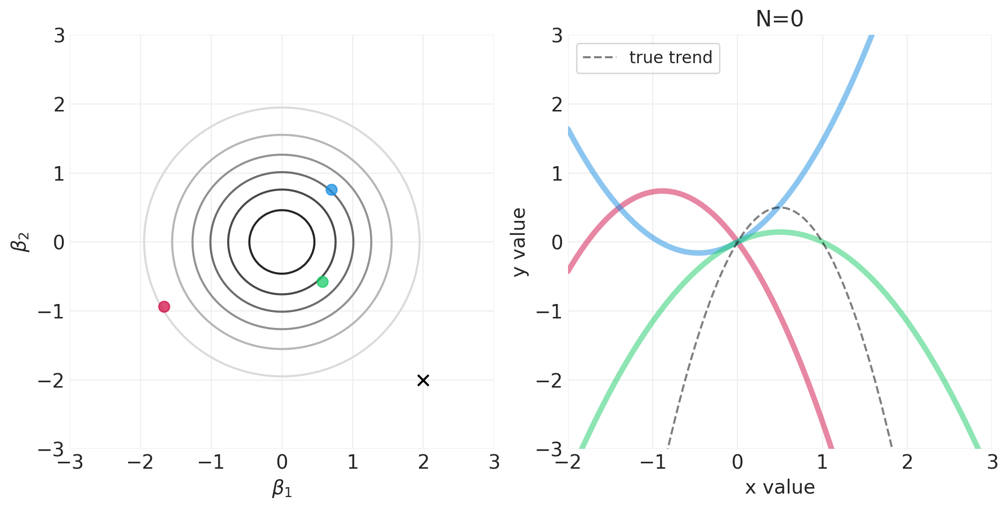
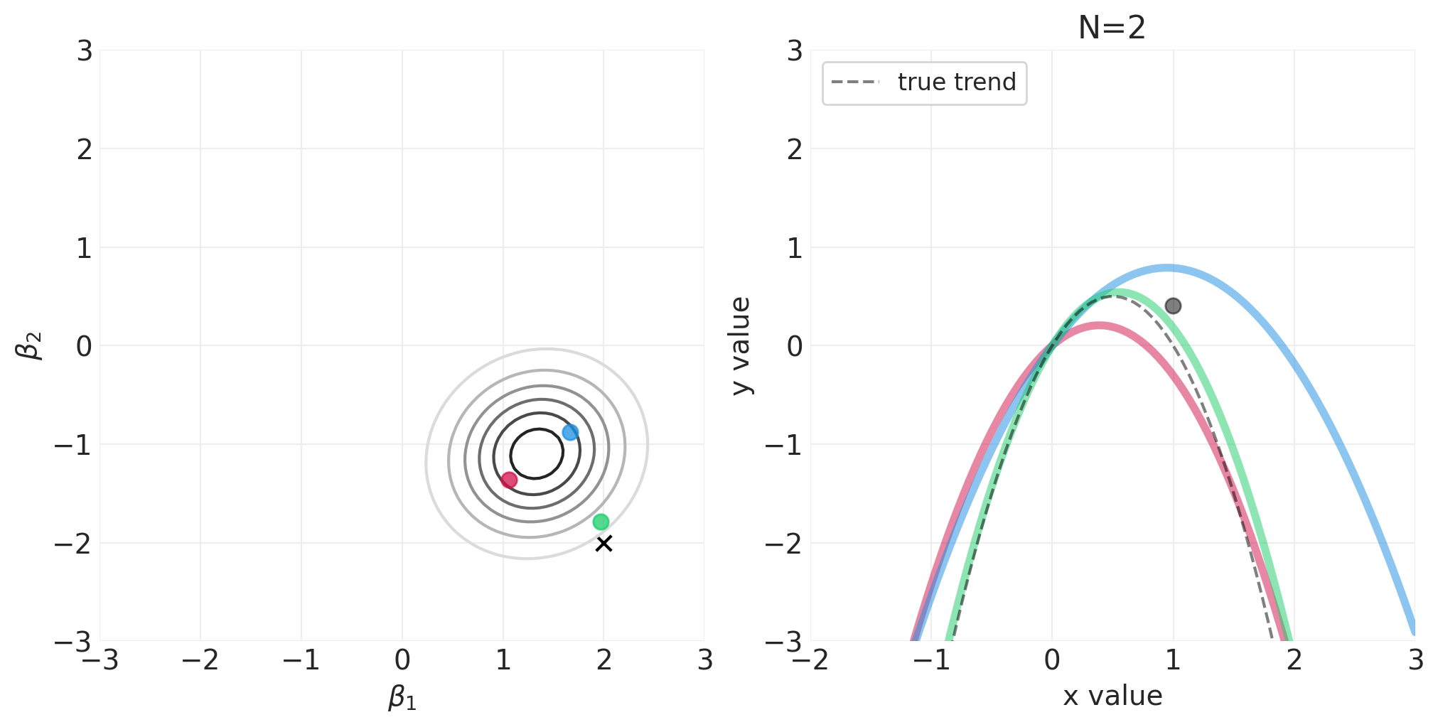
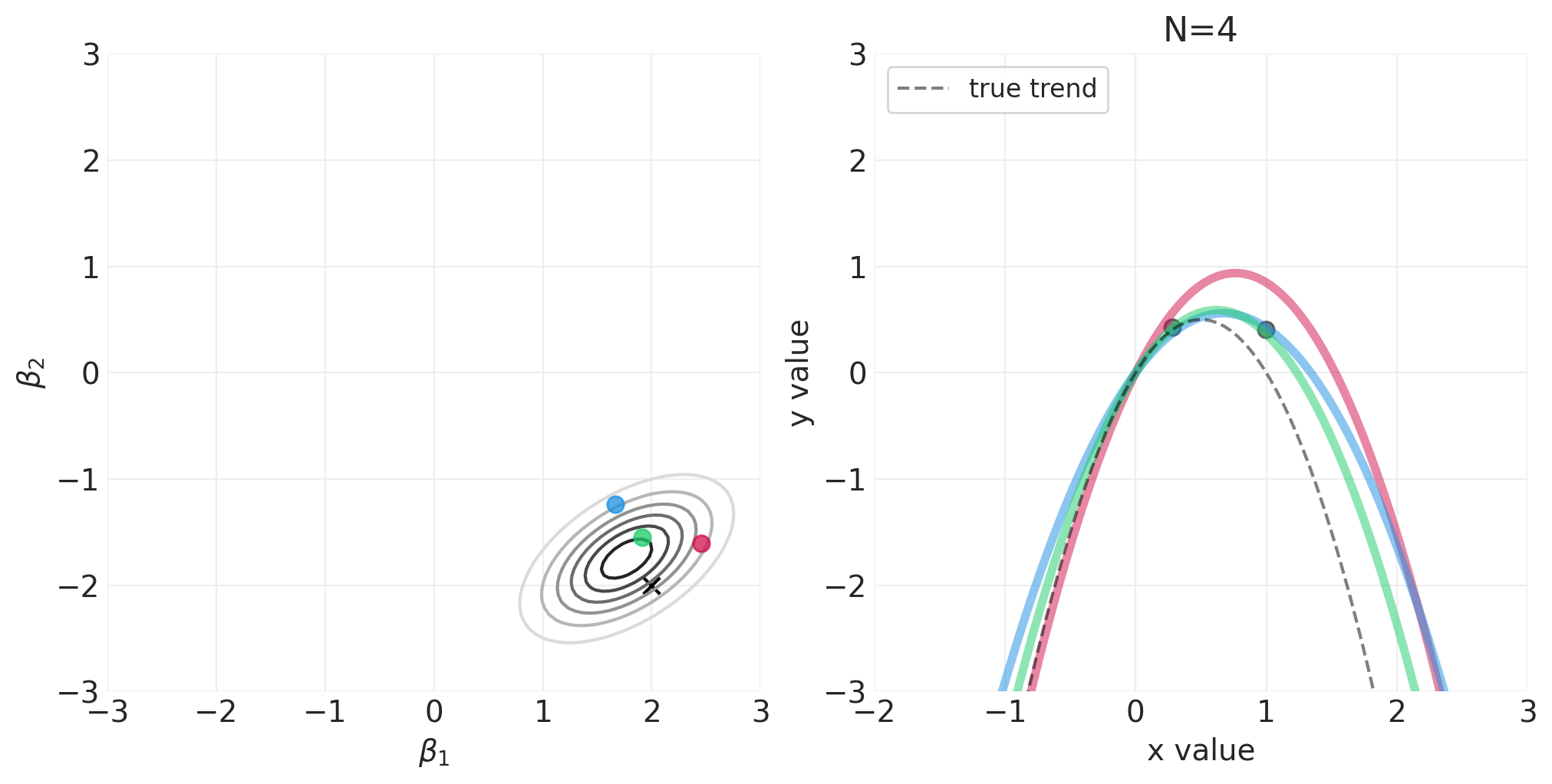
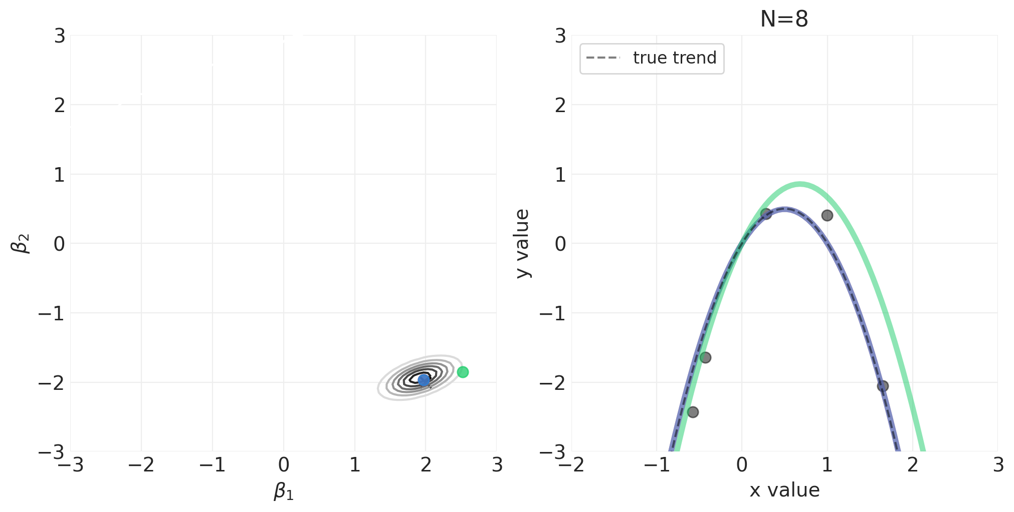
运行模拟

np.random.seed(123)
RESOLUTION = 100
N_DATA_POINTS = 64
BETA_1 = 2
BETA_2 = -2
INTERCEPT = 0

# Generate observations
x = stats.norm().rvs(size=N_DATA_POINTS)
y = INTERCEPT + BETA_1 * x + BETA_2 * x**2 + stats.norm.rvs(size=N_DATA_POINTS) * 0.5

beta_1_grid = np.linspace(-3, 3, RESOLUTION)
beta_2_grid = np.linspace(-3, 3, RESOLUTION)

# Vary the sample size to show how the posterior adapts to more and more data
for n_samples in [0, 2, 4, 8, 16, 32, 64]:

    utils.simulate_2_parameter_bayesian_learning_grid_approximation(
        x_obs=x[:n_samples],
        y_obs=y[:n_samples],
        param_a_grid=beta_1_grid,
        param_b_grid=beta_2_grid,
        true_param_a=BETA_1,
        true_param_b=BETA_2,
        model_func=quadratic_polynomial_model,
        posterior_func=quadratic_polynomial_regression_posterior,
        param_labels=["$\\beta_1$", "$\\beta_2$"],
        data_range_x=(-2, 3),
        data_range_y=(-3, 3),
    )

将 N 阶多项式拟合到身高/宽度数据

def fit_nth_order_polynomial(data, n=3):
    with pm.Model() as model:
        # Data
        H_std = pm.Data("H", utils.standardize(data.height.values), dims="obs_ids")

        # Priors
        sigma = pm.Uniform("sigma", 0, 10)
        alpha = pm.Normal("alpha", 0, 60)
        betas = []
        for ii in range(n):
            betas.append(pm.Normal(f"beta_{ii+1}", 0, 5))

        # Likelihood
        mu = alpha
        for ii, beta in enumerate(betas):
            mu += beta * H_std ** (ii + 1)

        mu = pm.Deterministic("mu", mu)

        pm.Normal("W_obs", mu, sigma, observed=data.weight.values, dims="obs_ids")

        inference = pm.sample(target_accept=0.95)

    return model, inference


polynomial_models = {}
for order in [2, 4, 6]:
    polynomial_models[order] = fit_nth_order_polynomial(HOWELL, n=order)

Initializing NUTS using jitter+adapt_diag...
Multiprocess sampling (4 chains in 4 jobs)
NUTS: [sigma, alpha, beta_1, beta_2]

Sampling 4 chains for 1_000 tune and 1_000 draw iterations (4_000 + 4_000 draws total) took 2 seconds.
Initializing NUTS using jitter+adapt_diag...
Multiprocess sampling (4 chains in 4 jobs)
NUTS: [sigma, alpha, beta_1, beta_2, beta_3, beta_4]

Sampling 4 chains for 1_000 tune and 1_000 draw iterations (4_000 + 4_000 draws total) took 6 seconds.
Initializing NUTS using jitter+adapt_diag...
Multiprocess sampling (4 chains in 4 jobs)
NUTS: [sigma, alpha, beta_1, beta_2, beta_3, beta_4, beta_5, beta_6]

Sampling 4 chains for 1_000 tune and 1_000 draw iterations (4_000 + 4_000 draws total) took 48 seconds.

def plot_polynomial_model_posterior_predictive(model, inference, data, order):

    # Sample the posterior predictive for regions outside of the training data
    prediction_heights = np.linspace(30, 200, 100)
    with model:
        std_heights = (prediction_heights - data.height.mean()) / data.height.std()
        pm.set_data({"H": std_heights})
        ppd = pm.sample_posterior_predictive(inference, extend_inferencedata=False)

    plt.subplots(figsize=(4, 4))
    plt.scatter(data.height, data.weight)
    az.plot_hdi(
        prediction_heights,
        ppd.posterior_predictive["W_obs"],
        color="k",
        fill_kwargs=dict(alpha=0.1),
    )

    # Hack: use .5% HDI as proxy for posterior predictive mean
    az.plot_hdi(
        prediction_heights,
        ppd.posterior_predictive["W_obs"],
        hdi_prob=0.005,
        color="k",
        fill_kwargs=dict(alpha=1),
    )
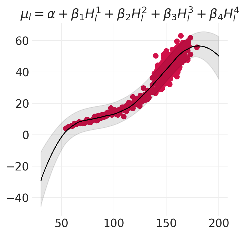
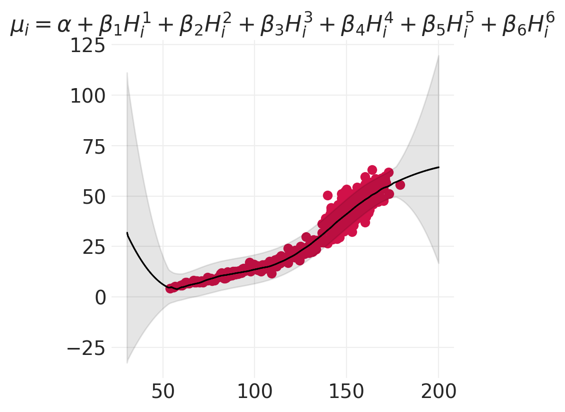
    terms = "+".join([f"\\beta_{o} H_i^{o}" for o in range(1, order + 1)])
    plt.title(f"$\mu_i = \\alpha + {terms}$")


for order in [2, 4, 6]:
    model, inference = polynomial_models[order]
    plot_polynomial_model_posterior_predictive(model, inference, HOWELL, order)

Sampling: [W_obs]

Sampling: [W_obs]

Sampling: [W_obs]

思考 vs 拟合

• 线性模型可以拟合任何事物（地心说）

• 最好使用领域专业知识来构建更符合生物学原理的模型，例如

\[\begin{split} \begin{align*} \log W_i = \text{Normal}(\mu_i, \sigma) \\ \mu_i = \alpha + \beta (H - \bar H) \end{align*} \end{split}\]

样条

• “摆动”由局部拟合的平滑函数构建

• 当您对问题领域知识了解甚少时，是不错的替代方案

\[ \mu_i = \alpha_0 + \alpha_1 B_1 + \alpha_2 B_2 + ... \alpha_S B_K \]

其中 \(B\) 是一组 \(K\) 局部核函数

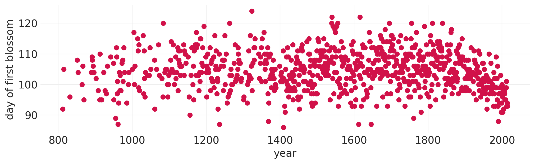
示例：樱花盛开

BLOSSOMS = utils.load_data("cherry_blossoms")
BLOSSOMS.dropna(subset=["doy"], inplace=True)
plt.subplots(figsize=(10, 3))
plt.scatter(x=BLOSSOMS.year, y=BLOSSOMS.doy)
plt.xlabel("year")
plt.ylabel("day of first blossom")
BLOSSOMS.head()

	年份	doy	温度	temp_upper	temp_lower
11	812	92.0	NaN	NaN	NaN
14	815	105.0	NaN	NaN	NaN
30	831	96.0	NaN	NaN	NaN
50	851	108.0	7.38	12.1	2.66
52	853	104.0	NaN	NaN	NaN

from patsy import dmatrix


def generate_spline_basis(data, xdim="year", degree=2, n_bases=10):
    n_knots = n_bases - 1
    knots = np.quantile(data[xdim], np.linspace(0, 1, n_knots))
    return dmatrix(
        f"bs({xdim}, knots=knots, degree={degree}, include_intercept=True) - 1",
        {xdim: data[xdim], "knots": knots[1:-1]},
    )


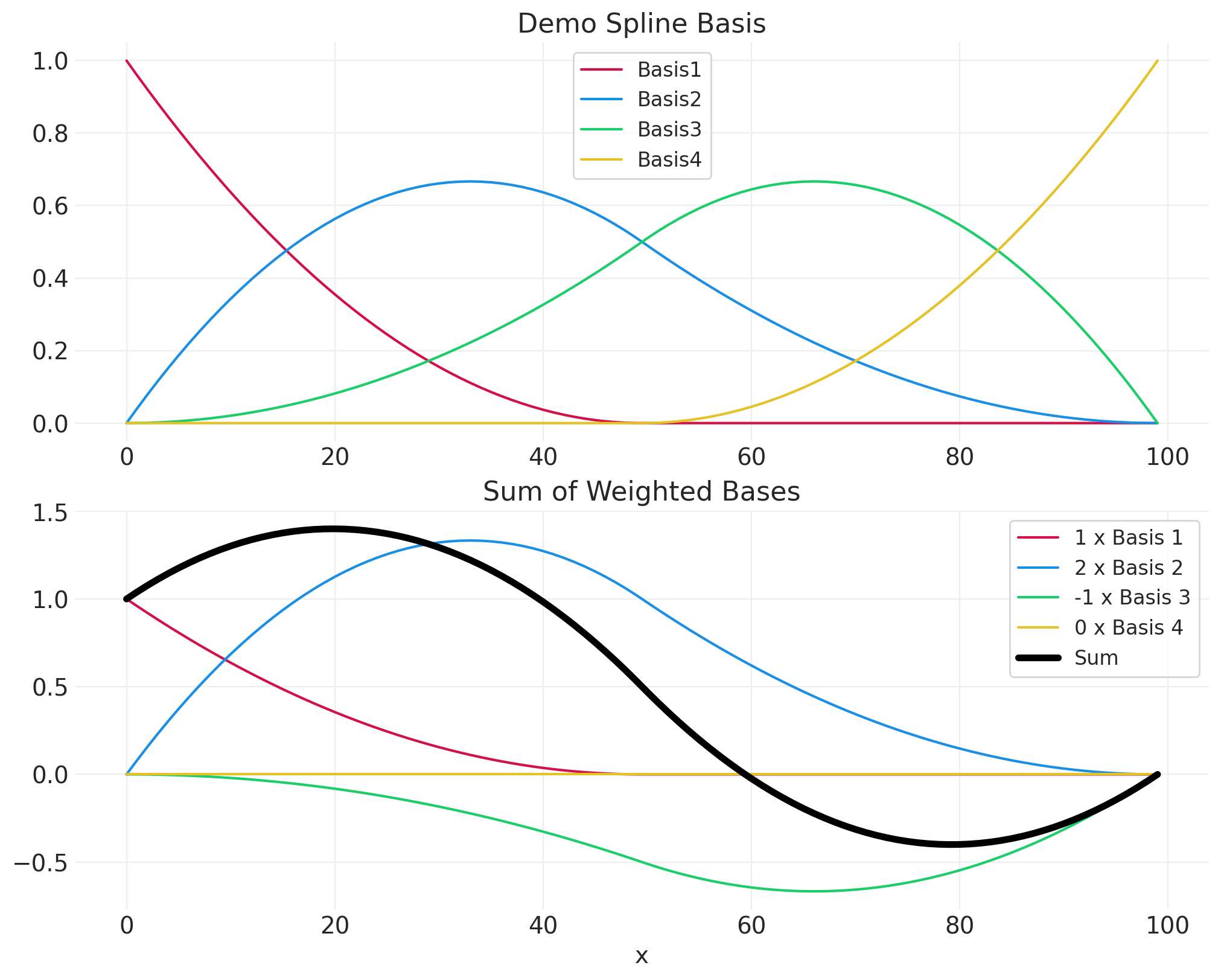
# 4 spline basis for demo
demo_data = pd.DataFrame({"x": np.arange(100)})
demo_basis = generate_spline_basis(demo_data, "x", n_bases=4)

fig, axs = plt.subplots(2, 1, figsize=(10, 8))
plt.sca(axs[0])
for bi in range(demo_basis.shape[1]):
    plt.plot(demo_data.x, demo_basis[:, bi], color=f"C{bi}", label=f"Basis{bi+1}")
plt.legend()
plt.title("Demo Spline Basis")

# Arbitrarily-set weights for demo
basis_weights = [1, 2, -1, 0]

plt.sca(axs[1])
resulting_curve = np.zeros_like(demo_data.x)
for bi in range(demo_basis.shape[1]):
    weighted_basis = demo_basis[:, bi] * basis_weights[bi]
    resulting_curve = resulting_curve + weighted_basis
    plt.plot(
        demo_data.x, weighted_basis, color=f"C{bi}", label=f"{basis_weights[bi]} x Basis {bi+1}"
    )
plt.plot(demo_data.x, resulting_curve, label="Sum", color="k", linewidth=4)
plt.xlabel("x")
plt.legend()
plt.title("Sum of Weighted Bases");

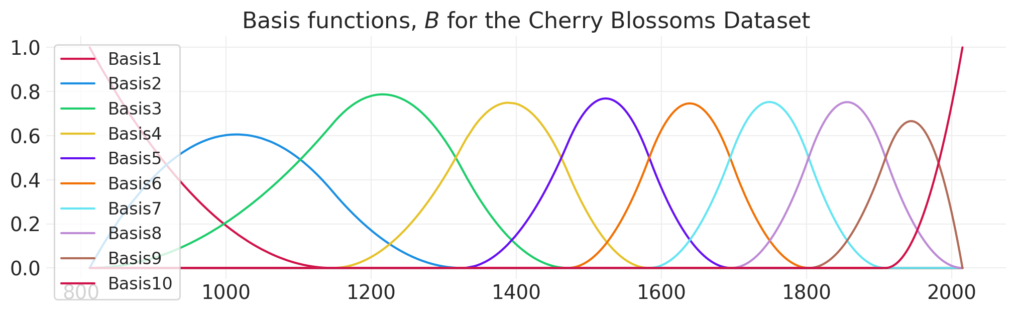
# 10 spline basis for modeling blossoms data
blossom_basis = generate_spline_basis(BLOSSOMS)

fig, ax = plt.subplots(figsize=(10, 3))

for bi in range(blossom_basis.shape[1]):
    ax.plot(BLOSSOMS.year, blossom_basis[:, bi], color=f"C{bi}", label=f"Basis{bi+1}")
plt.legend()
plt.title("Basis functions, $B$ for the Cherry Blossoms Dataset");

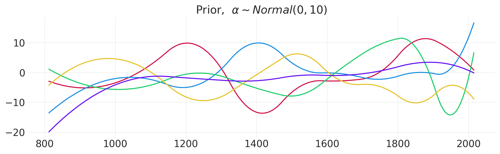
从先验中抽取一些样本

fig, ax = plt.subplots(figsize=(10, 3))
n_samples = 5
spline_prior_sigma = 10
spline_prior = stats.norm(0, spline_prior_sigma)
for s in range(n_samples):
    sample = 0
    for bi in range(blossom_basis.shape[1]):
        sample += spline_prior.rvs() * blossom_basis[:, bi]
    ax.plot(BLOSSOMS.year, sample)
plt.title("Prior,  $\\alpha \\sim Normal(0, 10)$");

def fit_spline_model(data, xdim, ydim, n_bases=10):
    basis_set = generate_spline_basis(data, xdim, n_bases=n_bases).base
    with pm.Model() as spline_model:

        # Priors
        sigma = pm.Exponential("sigma", 1)
        alpha = pm.Normal("alpha", data[ydim].mean(), data[ydim].std())
        beta = pm.Normal("beta", 0, 25, shape=n_bases)

        # Likelihood
        mu = pm.Deterministic("mu", alpha + pm.math.dot(basis_set, beta.T))
        pm.Normal("ydim_obs", mu, sigma, observed=data[ydim].values)

        spline_inference = pm.sample(target_accept=0.95)

    _, ax = plt.subplots(figsize=(10, 3))
    plt.scatter(x=data[xdim], y=data[ydim])
    az.plot_hdi(
        data[xdim],
        spline_inference.posterior["mu"],
        color="k",
        hdi_prob=0.89,
        fill_kwargs=dict(alpha=0.3, label="Posterior Mean"),
    )
    plt.legend(loc="lower right")
    plt.xlabel(f"{xdim}")
    plt.ylabel(f"{ydim}")

    return spline_model, spline_inference, basis_set

樱花模型

blossom_model, blossom_inference, blossom_basis = fit_spline_model(
    BLOSSOMS, "year", "doy", n_bases=20
)

Initializing NUTS using jitter+adapt_diag...
Multiprocess sampling (4 chains in 4 jobs)
NUTS: [sigma, alpha, beta]

Sampling 4 chains for 1_000 tune and 1_000 draw iterations (4_000 + 4_000 draws total) took 7 seconds.
The rhat statistic is larger than 1.01 for some parameters. This indicates problems during sampling. See https://arxiv.org/abs/1903.08008 for details
The effective sample size per chain is smaller than 100 for some parameters.  A higher number is needed for reliable rhat and ess computation. See https://arxiv.org/abs/1903.08008 for details

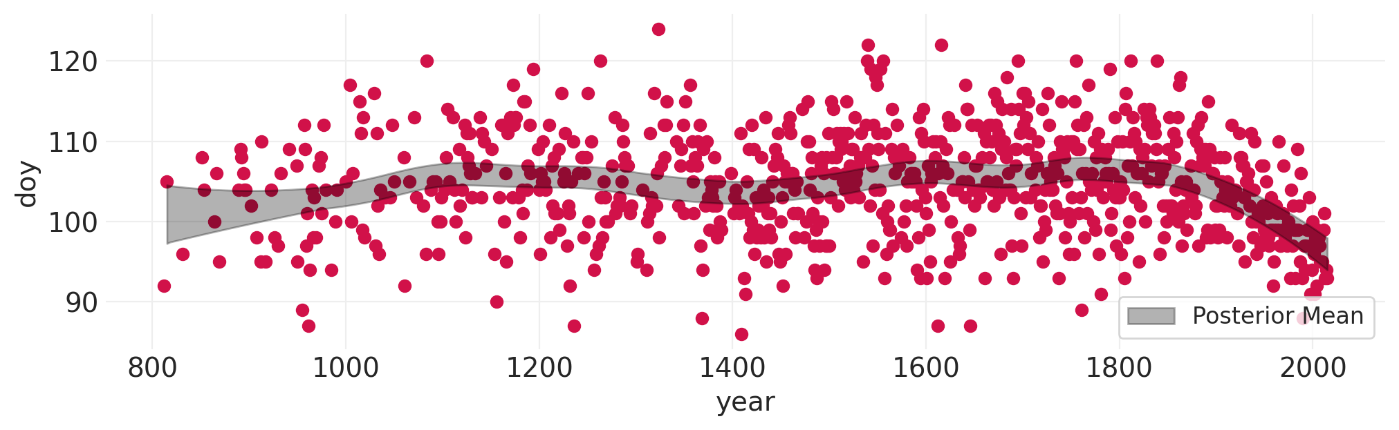
summary = az.summary(blossom_inference, var_names=["alpha", "beta"])

beta_spline_mean = blossom_inference.posterior["beta"].mean(dim=("chain", "draw")).values
resulting_fit = np.zeros_like(BLOSSOMS.year)
for bi, beta in enumerate(beta_spline_mean):
    weighted_basis = beta * blossom_basis[:, bi]
    plt.plot(BLOSSOMS.year, weighted_basis, color=f"C{bi}")
    resulting_fit = resulting_fit + weighted_basis
plt.plot(
    BLOSSOMS.year,
    resulting_fit,
    label="Resulting Fit (excluding intercept term)",
    color="k",
    linewidth=4,
)
plt.legend()
plt.title("weighted spline bases\nfit to Cherry Blossoms dataset")

summary

	均值	标准差	hdi_3%	hdi_97%	mcse_mean	mcse_sd	ess_bulk	ess_tail	r_hat
alpha	104.169	4.159	95.990	111.727	0.250	0.177	281.0	439.0	1.02
beta[0]	-3.632	5.052	-13.404	5.570	0.259	0.191	382.0	670.0	1.01
beta[1]	-1.924	4.706	-10.583	6.904	0.250	0.177	355.0	529.0	1.01
beta[2]	-0.097	4.455	-7.606	9.023	0.255	0.180	312.0	541.0	1.01
beta[3]	4.268	4.350	-3.914	12.500	0.248	0.181	310.0	443.0	1.01
beta[4]	-2.436	4.429	-10.230	6.570	0.263	0.186	286.0	468.0	1.01
beta[5]	4.529	4.436	-3.403	13.299	0.246	0.182	326.0	433.0	1.01
beta[6]	-3.418	4.413	-11.114	5.604	0.249	0.176	316.0	551.0	1.01
beta[7]	-1.262	4.426	-9.130	7.628	0.251	0.212	312.0	455.0	1.01
beta[8]	2.271	4.356	-5.789	10.885	0.247	0.175	311.0	490.0	1.01
beta[9]	4.240	4.431	-3.503	13.088	0.246	0.182	326.0	466.0	1.01
beta[10]	-2.424	4.396	-10.942	5.742	0.250	0.177	314.0	458.0	1.01
beta[11]	3.684	4.392	-4.651	11.830	0.257	0.182	293.0	513.0	1.01
beta[12]	2.999	4.425	-5.131	11.591	0.252	0.178	314.0	482.0	1.01
beta[13]	0.109	4.416	-7.990	8.775	0.249	0.176	316.0	493.0	1.01
beta[14]	2.393	4.407	-5.911	10.555	0.257	0.182	298.0	389.0	1.01
beta[15]	2.963	4.424	-5.112	11.599	0.253	0.179	310.0	552.0	1.01
beta[16]	0.342	4.397	-7.992	8.469	0.247	0.175	322.0	549.0	1.01
beta[17]	-1.831	4.463	-10.088	6.757	0.260	0.184	295.0	475.0	1.01
beta[18]	-7.074	4.628	-15.747	1.437	0.250	0.177	345.0	557.0	1.01
beta[19]	-8.827	4.638	-17.253	0.281	0.253	0.179	338.0	623.0	1.01

返回 Howell 数据集：使用样条模型将身高作为年龄的函数

# Fit spline model to Howell height data
fit_spline_model(HOWELL, "age", "height", n_bases=10);

Initializing NUTS using jitter+adapt_diag...
Multiprocess sampling (4 chains in 4 jobs)
NUTS: [sigma, alpha, beta]

Sampling 4 chains for 1_000 tune and 1_000 draw iterations (4_000 + 4_000 draws total) took 6 seconds.
The rhat statistic is larger than 1.01 for some parameters. This indicates problems during sampling. See https://arxiv.org/abs/1903.08008 for details
The effective sample size per chain is smaller than 100 for some parameters.  A higher number is needed for reliable rhat and ess computation. See https://arxiv.org/abs/1903.08008 for details

体重作为年龄的函数

# While we're at it, let's fit spline model to Howell weight data
fit_spline_model(HOWELL, "age", "weight", n_bases=10);

Initializing NUTS using jitter+adapt_diag...
Multiprocess sampling (4 chains in 4 jobs)
NUTS: [sigma, alpha, beta]

Sampling 4 chains for 1_000 tune and 1_000 draw iterations (4_000 + 4_000 draws total) took 9 seconds.
The effective sample size per chain is smaller than 100 for some parameters.  A higher number is needed for reliable rhat and ess computation. See https://arxiv.org/abs/1903.08008 for details

# ...how about height as a function of weight
fit_spline_model(HOWELL, "height", "weight", n_bases=10);

Initializing NUTS using jitter+adapt_diag...
Multiprocess sampling (4 chains in 4 jobs)
NUTS: [sigma, alpha, beta]

Sampling 4 chains for 1_000 tune and 1_000 draw iterations (4_000 + 4_000 draws total) took 9 seconds.
The rhat statistic is larger than 1.01 for some parameters. This indicates problems during sampling. See https://arxiv.org/abs/1903.08008 for details

奖励：完整豪华贝叶斯

• 方法：将整个生成过程编程到一个模型中

• 包括多个子模型（即多个似然函数）

我们为什么要这样做？

• 汇总系统中的模型

• 可以从完整的生成模型运行模拟（干预）以查看因果估计。

utils.draw_causal_graph(edge_list=[("H", "W"), ("S", "H"), ("S", "W")], graph_direction="LR")

SEX_ID, SEX = pd.factorize(["M" if s else "F" for s in ADULT_HOWELL["male"].values])
with pm.Model(coords={"SEX": SEX}) as flb_model:

    # Data
    S = pm.Data("S", SEX_ID)
    H = pm.Data("H", ADULT_HOWELL.height.values)
    Hbar = pm.Data("Hbar", ADULT_HOWELL.height.mean())

    # Height Model
    ## Height priors
    tau = pm.Uniform("tau", 0, 10)
    h = pm.Normal("h", 160, 10, dims="SEX")
    nu = h[S]
    ## Height likelihood
    pm.Normal("H_obs", nu, tau, observed=ADULT_HOWELL.height.values)

    # Weight Model
    ## Weight priors
    alpha = pm.Normal("alpha", 60, 10, dims="SEX")
    beta = pm.Uniform("beta", 0, 1, dims="SEX")
    sigma = pm.Uniform("sigma", 0, 10)
    mu = alpha[S] + beta[S] * (H - Hbar)
    ## Weight likelihood
    pm.Normal("W_obs", mu, sigma, observed=ADULT_HOWELL.weight.values)

    flb_inference = pm.sample()

pm.model_to_graphviz(flb_model)

Initializing NUTS using jitter+adapt_diag...
Multiprocess sampling (4 chains in 4 jobs)
NUTS: [tau, h, alpha, beta, sigma]

Sampling 4 chains for 1_000 tune and 1_000 draw iterations (4_000 + 4_000 draws total) took 2 seconds.

flb_summary = az.summary(flb_inference)
flb_summary

	均值	标准差	hdi_3%	hdi_97%	mcse_mean	mcse_sd	ess_bulk	ess_tail	r_hat
alpha[M]	45.085	0.468	44.138	45.877	0.007	0.005	4889.0	3233.0	1.0
alpha[F]	45.193	0.443	44.364	46.011	0.007	0.005	4158.0	3105.0	1.0
beta[M]	0.612	0.057	0.506	0.718	0.001	0.001	4935.0	3019.0	1.0
beta[F]	0.662	0.062	0.545	0.777	0.001	0.001	4127.0	3035.0	1.0
h[M]	160.354	0.444	159.561	161.188	0.006	0.004	6012.0	3206.0	1.0
h[F]	149.533	0.408	148.753	150.292	0.006	0.004	5042.0	3045.0	1.0
sigma	4.265	0.163	3.961	4.571	0.002	0.001	6503.0	3192.0	1.0
tau	5.555	0.213	5.175	5.960	0.003	0.002	5921.0	3096.0	1.0

使用 do 算子模拟干预

from pymc.model.transform.conditioning import do

def plot_posterior_mean_contrast(contrast_type="weight"):
    Hbar = ADULT_HOWELL.height.mean()
    means = az.summary(flb_inference)["mean"]

    H_F = stats.norm(means["h[F]"], means["tau"]).rvs(1000)
    H_M = stats.norm(means["h[M]"], means["tau"]).rvs(1000)

    W_F = stats.norm(means["beta[F]"] * (H_F - Hbar), means["sigma"]).rvs(1000)
    W_M = stats.norm(means["beta[M]"] * (H_M - Hbar), means["sigma"]).rvs(1000)
    contrast = H_M - H_F if contrast_type == "height" else W_M - W_F

    az.plot_dist(contrast, color="k")
    plt.xlabel(f"Posterior mean {contrast_type} contrast")


def plot_causal_intervention_contrast(contrast_type, intervention_type="pymc_do_operator"):
    N = len(ADULT_HOWELL)
    if intervention_type == "pymc_do_operator":
        male_counterfactual_data = {"S": np.ones(N, dtype="int32")}
        female_counterfactual_data = {"S": np.zeros(N, dtype="int32")}

        if contrast_type == "weight":
            contrast_variable = "W_obs"
            mean_heights = ADULT_HOWELL.groupby("male")["height"].mean()
            male_counterfactual_data.update({"H": np.ones(N) * mean_heights[1]})
            female_counterfactual_data.update({"H": np.ones(N) * mean_heights[0]})
        else:
            contrast_variable = "H_obs"

        # p(Y| do(S=1))
        male_intervention_model = do(flb_model, male_counterfactual_data)

        # p(Y | do(S=0))
        female_intervention_model = do(flb_model, female_counterfactual_data)

        male_intervention_inference = pm.sample_posterior_predictive(
            flb_inference, model=male_intervention_model, predictions=True
        )
        female_intervention_inference = pm.sample_posterior_predictive(
            flb_inference, model=female_intervention_model, predictions=True
        )
        intervention_contrast = (
            male_intervention_inference.predictions - female_intervention_inference.predictions
        )
        contrast = intervention_contrast[contrast_variable]
    else:
        # Intervention by hand, like outlined in lecture
        Hbar = ADULT_HOWELL.height.mean()

        F_posterior = flb_inference.posterior.sel(SEX="F")
        M_posterior = flb_inference.posterior.sel(SEX="M")

        H_F = stats.norm.rvs(F_posterior["h"], F_posterior["tau"])
        H_M = stats.norm.rvs(M_posterior["h"], F_posterior["tau"])

        W_F = stats.norm.rvs(F_posterior["beta"] * (H_F - Hbar), F_posterior["sigma"])
        W_M = stats.norm.rvs(M_posterior["beta"] * (H_M - Hbar), M_posterior["sigma"])

        contrast = H_M - H_F if contrast_type == "height" else W_M - W_F

    pos_prob = 100 * np.sum(contrast >= 0) / np.product(contrast.shape)
    neg_prob = 100 - pos_prob

    kde_ax = az.plot_dist(contrast, color="k", plot_kwargs=dict(linewidth=3), bw=0.5)

    # Shade underneath posterior predictive contrast
    kde_x, kde_y = kde_ax.get_lines()[0].get_data()

    # Proportion of PPD contrast below zero
    neg_idx = kde_x < 0
    plt.fill_between(
        x=kde_x[neg_idx],
        y1=np.zeros(sum(neg_idx)),
        y2=kde_y[neg_idx],
        color="C0",
        label=f"{neg_prob:1.0f}%",
    )

    pos_idx = kde_x >= 0
    plt.fill_between(
        x=kde_x[pos_idx],
        y1=np.zeros(sum(pos_idx)),
        y2=kde_y[pos_idx],
        color="C1",
        label=f"{pos_prob:1.0f}%",
    )

    plt.axvline(0, color="k")
    plt.legend()
    plt.xlabel(f"{contrast_type} counterfactual contrast")


def plot_flb_contrasts(
    contrast_type="weight", intervention_type="pymc_do_operator", figsize=(8, 4)
):
    _, axs = plt.subplots(1, 2, figsize=figsize)
    plt.sca(axs[0])
    plot_posterior_mean_contrast(contrast_type)

    plt.sca(axs[1])
    plot_causal_intervention_contrast(contrast_type, intervention_type)

plot_flb_contrasts("weight")

Sampling: [H_obs, W_obs]

Sampling: [H_obs, W_obs]

作者

• 由 Dustin Stansbury (2024) 移植到 PyMC

• 基于 Richard McElreath 的 Statistical Rethinking (2023) 讲座

%load_ext watermark
%watermark -n -u -v -iv -w -p pytensor,aeppl,xarray

Last updated: Sun Jan 19 2025

Python implementation: CPython
Python version       : 3.12.5
IPython version      : 8.27.0

pytensor: 2.26.4
aeppl   : not installed
xarray  : 2024.7.0

xarray     : 2024.7.0
arviz      : 0.19.0
scipy      : 1.14.1
matplotlib : 3.9.2
pandas     : 2.2.2
numpy      : 1.26.4
pymc       : 5.19.1
patsy      : 0.5.6
statsmodels: 0.14.2

Watermark: 2.5.0

许可声明

此示例 галерея 中的所有笔记本均在 MIT 许可证 下提供，该许可证允许修改和再分发以用于任何用途，前提是保留版权和许可声明。

引用 PyMC 示例

要引用此笔记本，请使用 Zenodo 为 pymc-examples 存储库提供的 DOI。

重要提示

许多笔记本都改编自其他来源：博客、书籍…… 在这种情况下，您也应该引用原始来源。

另请记住引用您的代码使用的相关库。

这是一个 bibtex 中的引用模板

@incollection{citekey,
  author    = "<notebook authors, see above>",
  title     = "<notebook title>",
  editor    = "PyMC Team",
  booktitle = "PyMC examples",
  doi       = "10.5281/zenodo.5654871"
}

一旦渲染，它可能看起来像