拟合不足与过拟合#

此笔记本是 PyMC 移植的 Statistical Rethinking 2023 Richard McElreath 讲座系列的一部分。

视频 - 第 07 讲 - 拟合不足与过拟合# 第 07 讲 - 拟合不足与过拟合

# Ignore warnings
import warnings

import arviz as az
import numpy as np
import pandas as pd
import pymc as pm
import statsmodels.formula.api as smf
import utils as utils
import xarray as xr

from matplotlib import pyplot as plt
from matplotlib import style
from scipy import stats as stats

warnings.filterwarnings("ignore")

# Set matplotlib style
STYLE = "statistical-rethinking-2023.mplstyle"
style.use(STYLE)

无限原因，有限数据#

有无数个估计器可以解释给定的样本。
通常在简单性（简约性）和准确性之间存在权衡

两个同时进行的斗争#

因果关系：使用逻辑和因果假设来设计估计器；比较和对比替代模型
有限数据：如何使估计器工作
- 估计器的存在是不够的，拥有估计器并不意味着它实用或有可能进行估计
- 我们需要考虑围绕估计的工程因素

预测问题#

创建玩具大脑体积数据集#

species = ["afarensis", "africanus", "habilis", "boisei", "rudolfensis", "ergaster", "sapiens"]
brain_volume_cc = [438, 452, 612, 521, 752, 871, 1350]
mass_kg = [37.0, 35.5, 34.5, 41.5, 55.5, 61.0, 53.5]

BRAIN_MASS_TOY = pd.DataFrame({"species": species, "brain": brain_volume_cc, "mass": mass_kg})

def plot_brain_mass_data(ax=None, data=BRAIN_MASS_TOY):
    if ax is not None:
        plt.sca(ax)
    utils.plot_scatter(data.mass, data.brain, color="k")
    plt.xlabel("mass (kg)")
    plt.ylabel("brain volume (cc)")


_, ax = plt.subplots(figsize=(4, 4))
plot_brain_mass_data(ax)

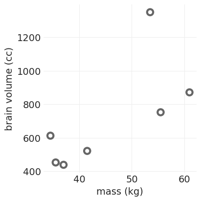
../_images/1a7b6c10b85208696ee82a6e57b11b69feab71139df8b3d0b4e19d936cef1402.png

考虑事项#

哪些可能的函数描述这些点
- 曲线拟合与压缩
哪些可能的函数解释这些点
- 这是因果推断的目标
如果我们改变其中一个点的质量会发生什么？
- 干预’
给定一个新的质量，相应的体积的期望值是多少
- 预测

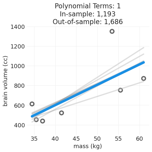
留一法交叉验证 (LOCCV)#

确定模型函数泛化能力的过程——即准确预测样本外数据点。

删除一个数据点
使用缺少的数据点拟合模型函数的参数
预测删除点的值，记录误差
对所有数据点重复 1-3
LOCCV 分数是所有删除点的误差总和

def fit_polynomial_cross_validated(order, data):
    n_data_points = len(data)
    data_idx = np.arange(n_data_points)
    params = []
    for ii in range(n_data_points):
        shift = n_data_points - 1 - ii
        cross_val_idx = sorted(np.roll(data_idx, shift)[: n_data_points - 1])

        cross_val_x = data.mass[cross_val_idx]
        cross_val_y = data.brain[cross_val_idx]
        cross_val_params = np.polyfit(cross_val_x, cross_val_y, order)
        params.append(cross_val_params)
    return np.array(params)


def estimate_n_degree_model_crossvalidated(order, data, ylims=(300, 1400)):
    cross_val_params = fit_polynomial_cross_validated(order, data)
    insample_model = np.poly1d(np.polyfit(data.mass, data.brain, order))

    ca = plt.gca()
    plot_brain_mass_data(ax=ca, data=data)

    out_of_sample_error = 0
    insample_error = 0

    xs = np.linspace(data.mass.min(), data.mass.max(), 100)
    for holdout_idx, params in enumerate(cross_val_params):

        model = np.poly1d(params)
        ys = model(xs)
        utils.plot_line(xs, ys, color="gray", label=None, alpha=0.25)

        holdout_x = data.loc[holdout_idx, "mass"]
        holdout_y = data.loc[holdout_idx, "brain"]

        holdout_prediction = model(holdout_x)
        insample_prediction = insample_model(holdout_x)

        # Here we use absolute error
        holdout_error = np.abs(holdout_prediction - holdout_y)
        insample_error_ = np.abs(insample_prediction - holdout_y)

        out_of_sample_error += holdout_error
        insample_error += insample_error_

    ys = insample_model(xs)
    utils.plot_line(xs, ys, color="C1", linewidth=6, label="Average Model")
    plt.ylim(ylims)
    plt.title(
        f"Polynomial Terms: {order}\nIn-sample: {insample_error:1,.0f}\nOut-of-sample: {out_of_sample_error:1,.0f}"
    )

    return insample_error, out_of_sample_error

plt.subplots(figsize=(5, 5))
insample_error, outsample_error = estimate_n_degree_model_crossvalidated(1, data=BRAIN_MASS_TOY)

../_images/a2eafd84a827b29870ae5e041735596182ed718fa5bbb429c6f4029ed326e3e0.png

使用 LO0CV 比较多项式模型#

def simulate_n_degree_polynomial_overfitting(data, ylims=(300, 1200)):

    fig, axs = plt.subplots(3, 2, figsize=(10, 12))
    insample_errors = []
    outsample_errors = []
    for ii in range(1, 6):
        row = (ii - 1) // 2
        col = (ii - 1) % 2
        plt.sca(axs[row, col])
        insample_error, outsample_error = estimate_n_degree_model_crossvalidated(
            ii, data=data, ylims=ylims
        )
        insample_errors.append(insample_error)
        outsample_errors.append(outsample_error)

    # rescale errors
    insample_errors = np.array(insample_errors)
    relative_insample_errors = insample_errors / insample_errors.sum()
    outsample_errors = np.array(outsample_errors)
    relative_outsample_errors = outsample_errors / outsample_errors.sum()

    plt.sca(axs[-1, -1])
    xs = np.arange(1, 6)

    utils.plot_line(xs, relative_insample_errors, color="C1", label="in-sample", alpha=1)
    utils.plot_scatter(
        xs, relative_insample_errors, color="C1", label=None, zorder=100, alpha=1, facecolors="w"
    )

    utils.plot_line(xs, relative_outsample_errors, color="C0", label="out-of-sample", alpha=1)
    utils.plot_scatter(
        xs, relative_outsample_errors, color="C0", label=None, zorder=100, alpha=1, facecolors="w"
    )
    plt.xlabel("polynomial terms")
    plt.ylabel("relative error")
    plt.legend()

    return outsample_errors, insample_errors

outsample_error, insample_error = simulate_n_degree_polynomial_overfitting(data=BRAIN_MASS_TOY);

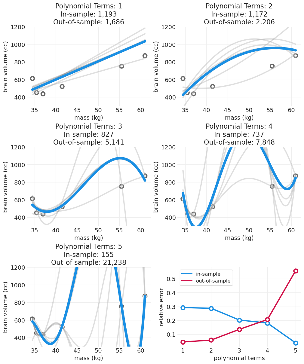
../_images/67cc43736527d46b33fc51f48e3d30f7c377446f57112922388d0909199ea63a.png

随着我们增加多项式阶数

样本内误差减少
样本外误差飙升
（至少对于简单模型）模型简单性和复杂性之间存在权衡，这反映在样本内和样本外误差的量上
模型复杂性中会存在一个“最佳点”，它足够复杂以拟合数据，但又不会过于复杂而过度拟合噪声。
这被称为偏差-方差权衡

注意这都适用于预测的目标，而不是因果推断。

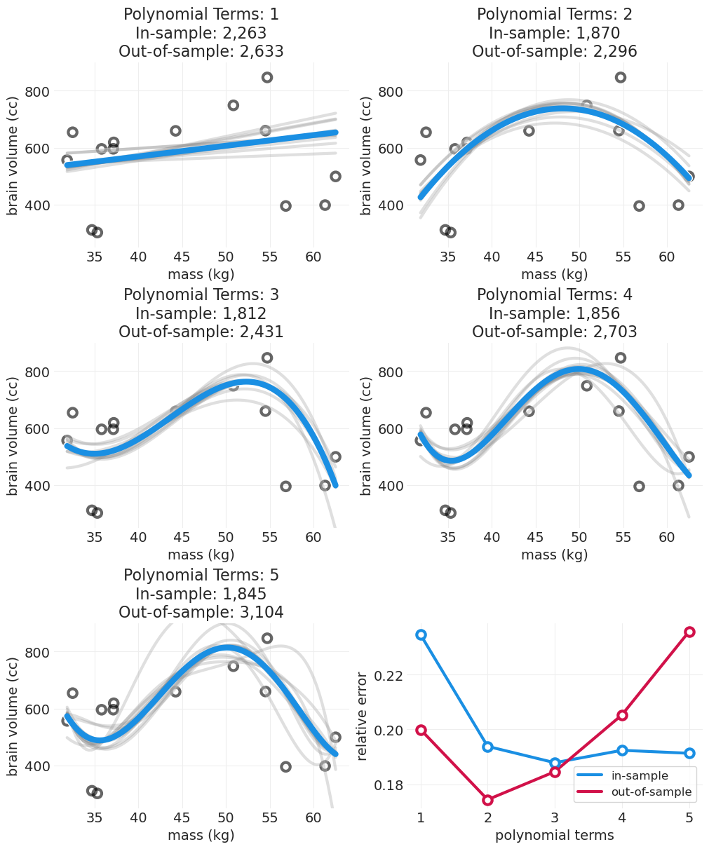
np.random.seed(1234)
n_samples = 15
# Run simulation with more data points
PRIMATE_DATA = utils.load_data("Primates301")[["brain", "body"]].dropna()

# preprocess the data a little
PRIMATE_DATA.loc[:, "brain"] = PRIMATE_DATA.brain * 10
PRIMATE_DATA.loc[:, "mass"] = PRIMATE_DATA.body / 100
PRIMATE_DATA = PRIMATE_DATA[PRIMATE_DATA.mass >= 30]
PRIMATE_DATA = PRIMATE_DATA[PRIMATE_DATA.mass <= 65]
PRIMATE_DATA = PRIMATE_DATA[PRIMATE_DATA.mass <= 900]

PRIMATE_DATA = PRIMATE_DATA.sample(n=n_samples).reset_index(drop=True)

np.random.seed(1234)
outsample_error, insample_error = simulate_n_degree_polynomial_overfitting(
    data=PRIMATE_DATA, ylims=(250, 900)
)

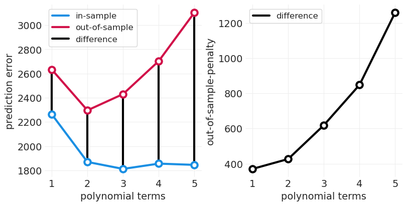
../_images/2e3544cea213deb6d0aaab9b345d3cbe402ee87a3399afedb4038dcf28d52583.png

def plot_out_of_sample_penalty(outsample_error, insample_error):
    penalty = outsample_error - insample_error
    n_terms = len(penalty)
    xs = np.arange(1, n_terms + 1)

    _, axs = plt.subplots(1, 2, figsize=(8, 4))
    plt.sca(axs[0])
    utils.plot_scatter(
        xs, insample_error, color="C1", label=None, zorder=100, alpha=1, facecolors="w"
    )
    utils.plot_line(xs, insample_error, color="C1", label="in-sample", alpha=1)

    utils.plot_scatter(
        xs, outsample_error, color="C0", label=None, zorder=100, alpha=1, facecolors="w"
    )
    utils.plot_line(xs, outsample_error, color="C0", label="out-of-sample", alpha=1)

    for ii, (out, inn) in enumerate(zip(outsample_error, insample_error)):
        label = "difference" if not ii else None
        plt.plot((ii + 1, ii + 1), (out, inn), color="k", lw=3, label=label)

    plt.ylabel("prediction error")
    plt.xlabel("polynomial terms")
    plt.legend()

    plt.sca(axs[1])
    utils.plot_scatter(xs, penalty, color="black", label=None, zorder=100, alpha=1, facecolors="w")
    utils.plot_line(xs, penalty, color="black", label="difference", alpha=1)
    plt.xlabel("polynomial terms")
    plt.xticks(xs)
    plt.ylabel("out-of-sample-penalty")
    plt.legend()


plot_out_of_sample_penalty(outsample_error, insample_error)

../_images/799d0b0893f0dbdc39a29b829cd1f1851a142c7d5c26b2fb39a0380b27b136b3.png

正则化#

模型灵活性和准确性之间将存在权衡。拥有过于灵活的模型可能导致过度加权噪声的贡献。
不希望您的估计器对罕见的异常值事件过于兴奋。您希望它找到常规特征。
贝叶斯建模使用更严格的先验（在方差方面），以便对不太可能的事件持怀疑态度，抑制估计器对异常值事件“兴奋”的倾向，从而降低模型对这些异常值建模的灵活性。
- 好的先验通常比人们想象的更严格
目标不是信号压缩（即记住数据的所有特征），而是预测中的泛化。

交叉验证不是正则化：CV 可用于比较模型，但不能降低灵活性（尽管我们可以平均模型）

正则化先验#

使用科学：领域知识是不可替代的
可以使用 CV 调整先验
许多任务是推断和预测的混合，因此权衡预测能力和做出可操作推断的能力

如果我们将样本外惩罚 (OOSP) 定义为样本外误差和样本内误差之间的差异，我们可以看到随着模型复杂性的增加，OOSP 也会增加。我们可以使用此指标通过为过度拟合提供信号来比较不同形式和复杂性的模型。

McElreath 继续展示贝叶斯交叉验证指标 WAIC 和 PSIS 与暴力 LOOCV（通过代理 lppd）返回的 OOSP 密切相关。在 Python/PyMC 中复制该图表会很好，但是，对于一个图表来说，这需要大量的额外编码和模型估计，所以我现在要跳过这一个。也就是说，我将在关于稳健回归的部分展示使用 PyMC 返回的 WAIC 和 PSIS 的示例。

惩罚预测和模型（错误）选择#

对于上面的简单示例，运行交叉验证以获得样本内和样本外惩罚没什么大不了的。但是，对于可能需要很长时间才能训练的更复杂模型，多次重新训练可能会令人望而却步。幸运的是，有一些 CV 程序的近似方法，允许我们直接从贝叶斯模型获得类似的指标，而无需显式运行 CV。这些指标包括

帕累托平滑重要性抽样 (PSIS)
Waikake 信息准则 (WAIC)

当直接解决因果推断问题时，不要使用 CV 惩罚来选择因果模型，这可能会导致选择一个混淆模型。混淆通常通过利用所有关联信号来帮助在没有干预的情况下进行预测。但是，在解决因果问题时，我们不想包含许多关联。

示例：模拟真菌生长#

以下是 McElreath v2 教材中代码 6.13 的翻译，用于模拟植物上的真菌生长。

utils.draw_causal_graph(
    edge_list=[("H0", "H1"), ("T", "H1"), ("T", "F"), ("F", "H1")],
    node_props={
        "T": {"label": "Treatment, T", "color": "red"},
        "F": {"label": "Fungus, F"},
        "H0": {"label": "Initial Height, H0"},
        "H1": {"label": "Final Height, H1"},
    },
    edge_props={
        ("T", "F"): {"color": "red"},
        ("F", "H1"): {"color": "red"},
        ("T", "H1"): {"color": "red"},
    },
)

../_images/7126cd0391f35cdc9122ed7d2bebb829dbeedb0a2d973ae5400bb09430a87aab.svg

模拟植物生长实验#

np.random.seed(12)

n_plants = 100

# Simulate initial heights
H0 = stats.norm.rvs(10, 2, size=n_plants)


# Treatment aids plant growth indirectly by reducing fungus,
# which has a negative effect on plant growth

# Simulate treatment
treatment = stats.bernoulli.rvs(p=0.5, size=n_plants)

# Simulate fungus growth conditioned on treatment
p_star = 0.5 - (treatment * 0.4)  # fungus is random when untreated, otherwise 10% chance
fungus = stats.bernoulli.rvs(p=p_star)

# Simulate final heights based on fungus
BETA_F = -3  # fungus hurts growth
ALPHA = 5
SIGMA = 1

mu = ALPHA + BETA_F * fungus
H1 = H0 + stats.norm.rvs(mu, SIGMA)

plants = pd.DataFrame(
    {"H0": H0, "treatment": treatment, "fungus": fungus, "H1": H1, "growth": H1 - H0}
)
plants.describe().T

	计数	平均值	标准差	最小值	25%	50%	75%	最大值
H0	100.0	9.711385	2.102440	3.705167	8.522114	9.779218	11.008820	15.743639
处理	100.0	0.550000	0.500000	0.000000	0.000000	1.000000	1.000000	1.000000
真菌	100.0	0.250000	0.435194	0.000000	0.000000	0.000000	0.250000	1.000000
H1	100.0	14.040887	2.587388	8.749880	12.286543	13.830425	15.764303	20.348779
生长	100.0	4.329502	1.719949	-0.604996	3.259297	4.824692	5.532195	7.533324

如果我们关注处理 \(T\) 对最终高度 \(H1\) 的总体因果影响

不正确的调整集（按 \(F\) 分层）#

\[\begin{split} \begin{align*} H_1 &\sim \mathcal{N}(\mu_i, \sigma) \\ \mu_i &= H_0 \times g_i \\ g_i &= \alpha + \beta_T T_i + \beta_F F_i \end{align*} \end{split}\]

结合了处理 \(T\) 和真菌 \(F\)，这是一个后处理变量（对因果推断不利）
\(F\) 不会通过后门准则找到
但是，提供比不结合 \(F\) 更准确的预测

with pm.Model() as biased_model:
    # Priors
    sigma = pm.Exponential("sigma", 1)
    alpha = pm.LogNormal("alpha", 0.2)
    beta_T = pm.Normal("beta_T", 0, 0.5)
    beta_F = pm.Normal("beta_F", 0, 0.5)

    H0 = plants.H0.values
    H1 = plants.H1.values

    T = pm.Data("T", treatment.astype(float))
    F = pm.Data("F", fungus.astype(float))

    # proportional amount of growth
    g = alpha + beta_T * T + beta_F * F
    mu = g * H0

    # Likelihood
    pm.Normal("H1", mu, sigma, observed=H1)

    biased_inference = pm.sample(target_accept=0.95)
    pm.compute_log_likelihood(biased_inference)

pm.model_to_graphviz(biased_model)

Initializing NUTS using jitter+adapt_diag...
Multiprocess sampling (4 chains in 4 jobs)
NUTS: [sigma, alpha, beta_T, beta_F]

Sampling 4 chains for 1_000 tune and 1_000 draw iterations (4_000 + 4_000 draws total) took 1 seconds.

../_images/bfb2aef9e1974fa4379a6c00846a294325dca2c4f0549e58c033d0a3462f20b8.svg

正确的调整集（不按 \(F\) 分层）#

\[\begin{split} \begin{align*} H_1 &\sim \mathcal{N}(\mu_i, \sigma) \\ \mu_i &= H_0 \times g_i \\ g_i &= \alpha + \beta_T T_i \end{align*} \end{split}\]

仅包括处理 T
预测不太准确，尽管是正确的因果模型

with pm.Model() as unbiased_model:
    # Priors
    sigma = pm.Exponential("sigma", 1.0)
    alpha = pm.LogNormal("alpha", 0.2)
    beta_T = pm.Normal("beta_T", 0, 0.5)

    H0 = plants.H0.values
    H1 = plants.H1.values

    T = pm.Data("T", treatment.astype(float))
    F = pm.Data("F", fungus.astype(float))

    # proportional amount of growth
    g = alpha + beta_T * T
    mu = g * H0

    # Likelihood
    pm.Normal("H1", mu, sigma, observed=H1)

    unbiased_inference = pm.sample(target_accept=0.95)
    pm.compute_log_likelihood(unbiased_inference)

pm.model_to_graphviz(unbiased_model)

Initializing NUTS using jitter+adapt_diag...
Multiprocess sampling (4 chains in 4 jobs)
NUTS: [sigma, alpha, beta_T]

Sampling 4 chains for 1_000 tune and 1_000 draw iterations (4_000 + 4_000 draws total) took 1 seconds.

../_images/294cc636ad17bc8c5c04fa07be5c8498eb132bda8cc5b7c1eee8d7b711249a13.svg

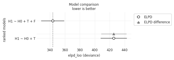
有偏差的模型提供更好的数据预测#

我们可以通过比较 LOO 交叉验证分数来看出，有偏差的模型排名更高

有偏差的模型权重 = 1
ELPD（偏差）较低（表明样本外预测更好）

comparison = az.compare(
    {"H1 ~ H0 + T + F": biased_inference, "H1 ~ H0 + T": unbiased_inference}, scale="deviance"
)
comparison

	排名	elpd_loo	p_loo	elpd_diff	权重	标准误差	标准误差差异	警告	比例
H1 ~ H0 + T + F	0	343.573135	4.186477	0.000000	1.000000e+00	15.426043	0.0000	假	偏差
H1 ~ H0 + T	1	425.412309	3.566714	81.839174	1.335820e-12	17.616036	16.9891	假	偏差

az.plot_compare(comparison, insample_dev=False);

../_images/253f8c26c9bc51324fdc1c72102ac4e98ed4e492cd96b5dba4f4ecf0fb15d7f1.png

但是，无偏差模型恢复了正确的因果效应#

az.summary(biased_inference)

	平均值	标准差	HDI_3%	HDI_97%	MCSE_均值	MCSE_标准差	ESS_批量	ESS_尾部	R_hat
Alpha	1.539	0.026	1.490	1.589	0.001	0.000	1833.0	2070.0	1.0
Beta_F	-0.362	0.033	-0.421	-0.299	0.001	0.001	2089.0	2454.0	1.0
Beta_T	-0.034	0.030	-0.086	0.022	0.001	0.000	1895.0	2390.0	1.0
Sigma	1.319	0.095	1.140	1.489	0.002	0.001	2539.0	2584.0	1.0

az.summary(unbiased_inference)

	平均值	标准差	HDI_3%	HDI_97%	MCSE_均值	MCSE_标准差	ESS_批量	ESS_尾部	R_hat
Alpha	1.369	0.032	1.308	1.426	0.001	0.001	1776.0	1806.0	1.0
Beta_T	0.091	0.041	0.015	0.171	0.001	0.001	1824.0	2052.0	1.0
Sigma	1.985	0.140	1.721	2.234	0.003	0.002	2366.0	2417.0	1.0

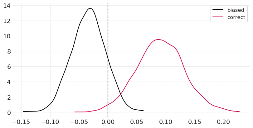
绘制每个模型的后验会提供不同的结果。有偏差的模型表明，处理对植物生长没有影响，甚至有负面影响。我们知道这不是真的，因为模拟要么对未处理组没有影响，要么对植物生长有积极影响（通过减少真菌间接实现）。

_, ax = plt.subplots(figsize=(8, 4))
az.plot_dist(biased_inference.posterior["beta_T"], ax=ax, color="black", label="biased")
az.plot_dist(unbiased_inference.posterior["beta_T"], ax=ax, color="C0", label="correct")
plt.axvline(0, linestyle="dashed", color="k");

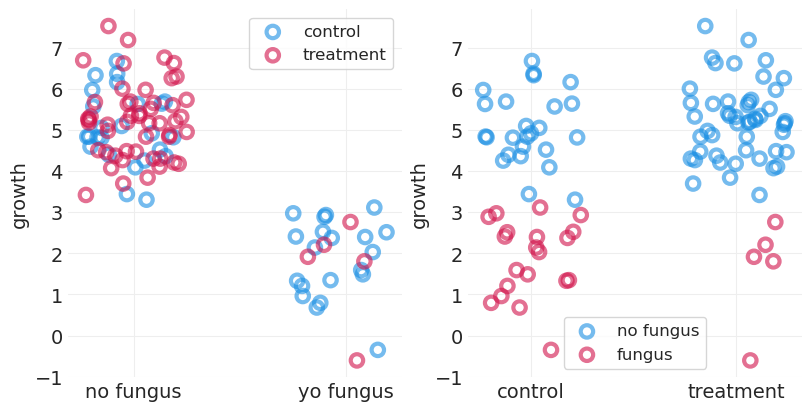
../_images/0a5194c20019d28f2d0dd7c6554ee0eebc0aaa14fd7f18eba24bade499067834.png

为什么错误的模型在预测中获胜？#

真菌是比处理更好的生长预测因子。
- 真菌和生长之间存在明显的（负）线性关系（下图左图）
  - 即，当按真菌分离时，边际分布更好分离
- 对照/处理提供的效果要差得多
  - 即，当按处理分割时，边际分布高度重叠
- 处理组中的真菌点较少（见下图右图）。这为评估处理和生长之间的预测关联提供了较少的训练集预测信号。

_, axs = plt.subplots(1, 2, figsize=(8, 4))

plt.sca(axs[0])
for treat, label in enumerate(["control", "treatment"]):
    plot_data = plants[plants.treatment == treat]
    jitter = 0.5 * (np.random.rand(len(plot_data)) - 0.5)
    color = f"C{np.abs(treat - 1)}"
    utils.plot_scatter(plot_data.fungus + jitter, plot_data.growth, color=color, label=label)

plt.xticks([0, 1], labels=["no fungus", "yo fungus"])
plt.legend()
plt.ylabel("growth")

plt.sca(axs[1])
for fungus, label in enumerate(["no fungus", "fungus"]):
    plot_data = plants[plants.fungus == fungus]
    jitter = 0.5 * (np.random.rand(len(plot_data)) - 0.5)
    color = f"C{np.abs(fungus - 1)}"
    utils.plot_scatter(plot_data.treatment + jitter, plot_data.growth, color=color, label=label)

plt.xticks([0, 1], labels=["control", "treatment"])
plt.ylabel("growth")

plt.legend();

../_images/a7df2237f13340d00569579cca5247cbce554db9d19e1bb5ea63143790528ed4.png

模型错误选择#

永远不要使用预测工具（WAIC、PSIS、CV/OOSPS）来选择因果估计
大多数分析都是预测和推断的混合。
准确的功能描述创建更简单、更简约的模型，这些模型不太容易过度拟合，因此尽可能使用科学

异常值和稳健回归#

异常值对后验的影响比“正常”点更大
- 您可以使用 CV 量化这一点——这与重要性抽样有关
不要删除异常值，它们仍然是信号
- 是模型错了，而不是数据
- 例如，混合模型和稳健回归

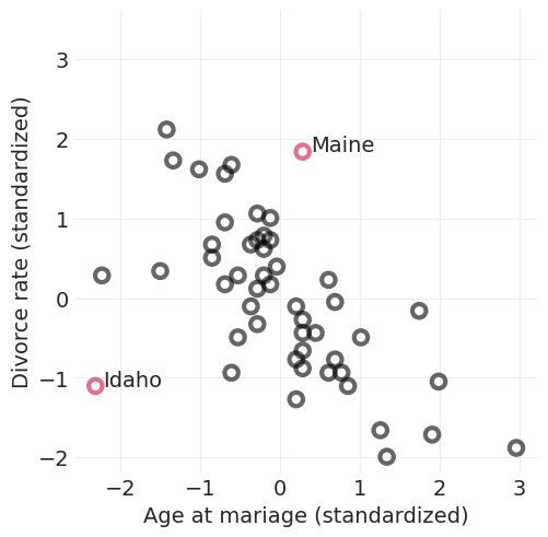
示例：离婚率#

缅因州和爱达荷州都很不寻常
缅因州：平均结婚年龄离婚率高
爱达荷州：离婚率低且结婚年龄低于平均水平

像爱达荷州和缅因州这样的异常值点的影响是什么？

divorce = utils.load_data("WaffleDivorce")[["Location", "Divorce", "MedianAgeMarriage"]]

inliers_idx = divorce.query("Location not in ('Idaho', 'Maine')").index.tolist()
outliers_idx = divorce.query("Location in ('Idaho', 'Maine')").index.tolist()


std_age = utils.standardize(divorce.MedianAgeMarriage)
std_divorce = utils.standardize(divorce.Divorce)

utils.plot_scatter(std_age[inliers_idx], std_divorce[inliers_idx], color="k", label=None)
utils.plot_scatter(std_age[outliers_idx], std_divorce[outliers_idx], color="C0", label=None)

for oi in outliers_idx:
    plt.annotate(divorce.loc[oi, "Location"], (std_age[oi] + 0.1, std_divorce[oi]), fontsize=14)

plt.xlabel("Age at mariage (standardized)")
plt.ylabel("Divorce rate (standardized)")
plt.axis("square");

../_images/d4963d29e46aaa6821a88cb2b87893e70ca55434192bf12701e7583dbf2536ee.png

拟合最小二乘模型#

with pm.Model() as lstsq_model:
    # Priors
    sigma = pm.Exponential("sigma", 1)
    alpha = pm.Normal("alpha", 0, 0.5)
    beta_A = pm.Normal("beta_A", 0, 0.5)

    # Likelihood
    mu = alpha + beta_A * std_age.values
    pm.Normal("divorce", mu, sigma, observed=std_divorce.values)
    lstsq_inference = pm.sample()

    # required for LOOCV score
    pm.compute_log_likelihood(lstsq_inference)

Initializing NUTS using jitter+adapt_diag...
Multiprocess sampling (4 chains in 4 jobs)
NUTS: [sigma, alpha, beta_A]

Sampling 4 chains for 1_000 tune and 1_000 draw iterations (4_000 + 4_000 draws total) took 1 seconds.

# Calculate Pointwise LOOCV scores
def plot_loocv(inference, title=None):
    plt.subplots(figsize=(6, 3))
    pareto_k = az.loo(inference, pointwise=True).pareto_k
    waic = -az.waic(inference, pointwise=True).waic_i

    utils.plot_scatter(pareto_k, waic, color="C0", label=None)
    for oi in outliers_idx:
        plt.annotate(divorce.loc[oi, "Location"], (pareto_k[oi] + 0.01, waic[oi]), fontsize=14)
    plt.xlabel("PSIS Pareto K")
    plt.ylabel("WAIC")
    plt.title(title)


plot_loocv(lstsq_inference, title="Gaussian Likelihood Posterior\nAffected by Outliers")

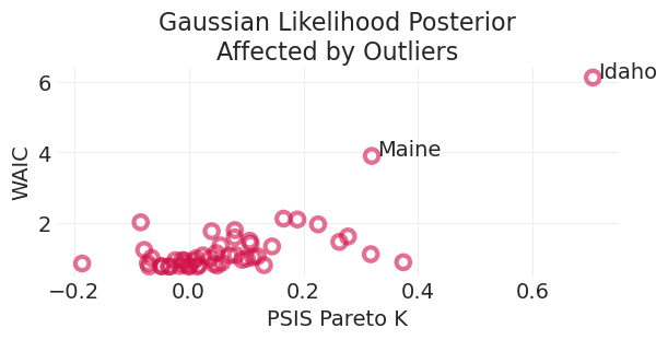
../_images/e8b09b97131d981b62d90b0f9be411057ca8a36b5dd6ed4c8a1ad213ca770b05.png

在这里我们可以看到，两个异常值对正态似然模型后验有很大影响。这是因为异常值在正态分布下的概率非常低，因此非常“令人惊讶”或“突出”。

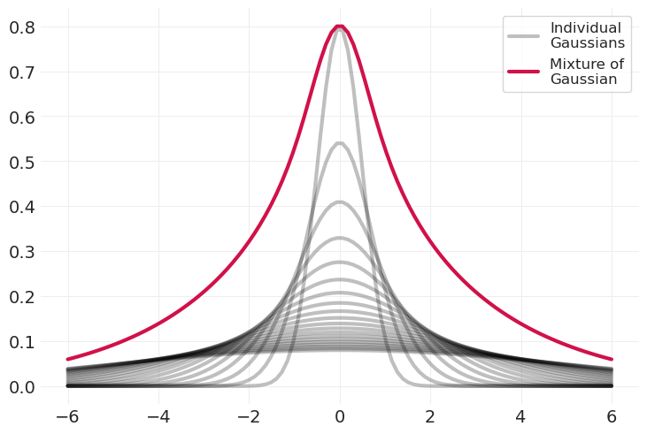
混合高斯分布——学生 t 分布#

添加不同方差的高斯分布会导致具有更肥尾的分布
隐含地捕获了人口中未观察到的异质性
- 多个重叠过程可能具有不同的方差。

xs = np.linspace(-6, 6, 100)
pdfs = []
n_gaussians = 20
for variance in np.linspace(0.5, 5, n_gaussians):
    label = "Individual\nGaussians" if variance == 0.5 else None
    pdf = stats.norm(0, variance).pdf(xs)
    pdfs.append(pdf)
    utils.plot_line(xs, pdf, color="k", label=label, alpha=0.25)

sum_of_pdfs = np.array(pdfs).sum(axis=0)
sum_of_pdfs /= sum_of_pdfs.max()
sum_of_pdfs *= 1 - n_gaussians / 100

utils.plot_line(xs, sum_of_pdfs, color="C0", label="Mixture of\nGaussian")
plt.legend();

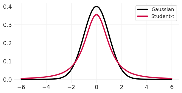
../_images/bb0d1bded74f215c1611fe4adc7ddfa30986130d72321b71e1d77830150938d3.png

plt.subplots(figsize=(6, 3))

utils.plot_line(xs, stats.norm.pdf(xs), color="k", label="Gaussian")
utils.plot_line(xs, stats.t(2).pdf(xs), color="C0", label="Student-t")
plt.legend();

../_images/250a0ad37ed42ab5a17f698990995edae1819ff9f904489655754de436f94c16.png

使用学生 t 似然的稳健线性回归#

with pm.Model() as studentt_model:
    # Priors
    sigma = pm.Exponential("sigma", 1)
    alpha = pm.Normal("alpha", 0, 0.5)
    beta_A = pm.Normal("beta_A", 0, 0.5)

    # Likelihood
    mu = alpha + beta_A * std_age.values
    # Replacing Gaussian with Student T -- note, we just "choose" 2 as our degrees of freedom
    pm.StudentT("divorce", nu=2, mu=mu, sigma=sigma, observed=std_divorce.values)
    studentt_inference = pm.sample()
    pm.compute_log_likelihood(studentt_inference)

Initializing NUTS using jitter+adapt_diag...
Multiprocess sampling (4 chains in 4 jobs)
NUTS: [sigma, alpha, beta_A]

Sampling 4 chains for 1_000 tune and 1_000 draw iterations (4_000 + 4_000 draws total) took 1 seconds.

plt.subplots(figsize=(6, 3))
az.plot_dist(lstsq_inference.posterior["beta_A"], color="k", label="Gaussian Model")
az.plot_dist(studentt_inference.posterior["beta_A"], color="C0", label="Student-t Model")
plt.xlabel("$\\beta_A$ (effect of age on divorce)")
plt.ylabel("density");

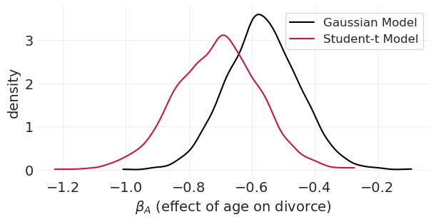
../_images/0b809c4c3953196ab6db4bae9b5d8764126ca917f386939673ba03735ce806d6.png

在这里我们可以看到，在普通的 Gaussian 线性回归中，异常值如何将后验拉得更靠近零。更稳健的学生 t 模型受这些异常值的影响较小。

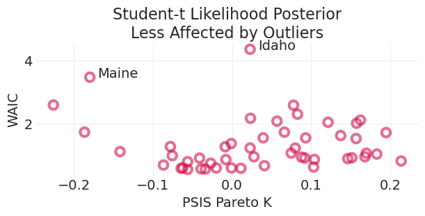
异常值对学生 t 后验的影响较小#

我们可以看到，使用对异常值更稳健的似然会减少这些异常值的权重，这由缅因州和爱达荷州给出的不太极端的后验重要性权重表示，特别是对于 PSIS。

plot_loocv(studentt_inference, title="Student-t Likelihood Posterior\nLess Affected by Outliers")

../_images/f0759515a0a68cdd655027ccd91298a5bc5034e51777c12d6dc88530b204ba63.png

回顾：稳健回归#

高斯混合/学生 t 隐含地捕获了人口中未观察到的异质性
这导致“厚尾”分布，这些分布对异常值“不太惊讶”
我们在学生 t 分布中“只需设置”自由度参数。事实证明，很难从数据中准确估计自由度，因为异常值很少见。
对于理论不足的领域，我们是否应该默认使用稳健回归？
- 可能是一个好主意
- 示例：自 1900 年代初期以来，世界变得更加和平。
  - 厚尾分布表明，像 1900 年代早期的那些大规模冲突并不令人惊讶，而是社会冲突等过程预期会发生的（这些过程往往是长尾的），这些冲突可能会加剧并“失控”。

作者#

移植到 PyMC：Dustin Stansbury (2024)
基于 Richard McElreath 的 Statistical Rethinking (2023) 讲座

%load_ext watermark
%watermark -n -u -v -iv -w -p pytensor,aeppl,xarray

Last updated: Tue Dec 17 2024

Python implementation: CPython
Python version       : 3.12.5
IPython version      : 8.27.0

pytensor: 2.26.4
aeppl   : not installed
xarray  : 2024.7.0

statsmodels: 0.14.2
scipy      : 1.14.1
xarray     : 2024.7.0
matplotlib : 3.9.2
numpy      : 1.26.4
pandas     : 2.2.2
pymc       : 5.19.1
arviz      : 0.19.0

Watermark: 2.5.0

许可声明#

此示例库中的所有笔记本均根据 MIT 许可证提供，该许可证允许修改和再分发以用于任何用途，前提是保留版权和许可声明。

引用 PyMC 示例#

要引用此笔记本，请使用 Zenodo 为 pymc-examples 存储库提供的 DOI。

重要提示

许多笔记本改编自其他来源：博客、书籍……在这种情况下，您也应该引用原始来源。

另请记住引用您的代码使用的相关库。

这是一个 bibtex 中的引用模板

@incollection{citekey,
  author    = "<notebook authors, see above>",
  title     = "<notebook title>",
  editor    = "PyMC Team",
  booktitle = "PyMC examples",
  doi       = "10.5281/zenodo.5654871"
}

一旦渲染，它可能看起来像

分类

标签