


马尔可夫链蒙特卡洛#
此笔记本是 PyMC 移植的 Statistical Rethinking 2023 Richard McElreath 讲座系列的一部分。
视频 - 第 08 讲 - 马尔可夫链蒙特卡洛# 第 08 讲 - 马尔可夫链蒙特卡洛
# Ignore warnings
import warnings

import arviz as az
import numpy as np
import pandas as pd
import pymc as pm
import statsmodels.formula.api as smf
import utils as utils
import xarray as xr

from matplotlib import pyplot as plt
from matplotlib import style
from scipy import stats as stats

warnings.filterwarnings("ignore")

# Set matplotlib style
STYLE = "statistical-rethinking-2023.mplstyle"
style.use(STYLE)
真实世界的研究#
真实世界是复杂的,需要更复杂的因果模型。利用随机数生成器的数值方法是(目前)估计更复杂因果模型的后验分布最实用的方法
由测量和噪声引起的复杂性#
示例:婚姻 & 离婚率数据集#
我们在第 07 讲中分析的图#
utils.draw_causal_graph(edge_list=[("M", "D"), ("A", "D"), ("A", "M")], graph_direction="LR")

然而,真实世界的图可能更加复杂#
utils.draw_causal_graph(
    edge_list=[
        ("A", "M"),
        ("A", "D"),
        ("A", "A*"),
        ("M", "M*"),
        ("D", "D*"),
        ("P", "A*"),
        ("P", "M*"),
        ("P", "D*"),
    ],
    node_props={
        "A": {"style": "dashed"},
        "D": {"style": "dashed"},
        "M": {"style": "dashed"},
        "unobserved": {"style": "dashed"},
    },
)

我们实际上没有直接观察到婚姻 \(M\)、离婚 \(D\) 和年龄 \(A\),而是观察到与每个 \(M*, D*, A*\) 相关的噪声测量。
除了测量噪声外,潜在人口 \(P\) 也会导致可靠性变化,这可能会影响我们对 \(M*, D*, A*\) 的估计(例如,较小的州观测值较少,因此估计的可靠性较低)。
由潜在的、未观察到的原因引起的复杂性#
示例:测试分数#
utils.draw_causal_graph(
    edge_list=[("K", "S"), ("X", "S"), ("X", "K"), ("Q", "S")],
    node_props={
        "K": {"style": "dashed"},
        "Q": {"style": "dashed"},
        "unobserved": {"style": "dashed"},
    },
    graph_direction="LR",
)

测试分数 \(S\) 是以下因素的函数
观察到的学生特征 \(X\)
未观察到的知识状态 \(K\)
测试质量/难度 \(Q\)
问题和解决方案#
真实世界研究中的其他复杂性#
以下因素会使计算后验变得困难
许多未知数和未观察到的变量
嵌套关系 – 到目前为止,模型或多或少是加法的,但情况并非总是如此
有界结果 – 应该具有有限支持的参数
难以计算后验
解析方法 – 我们很少能依赖闭式数学解(例如,共轭先验情景)
网格近似 – 仅适用于小型问题(维度诅咒)
二次近似 – 仅适用于部分问题(例如,多元高斯后验)
MCMC - 通用,但计算成本高昂 – 随着最近计算能力的提高,它变得更容易访问。
分析数据#
在这里,我们深入研究用于估计工作流估计阶段后验的黑匣子。
计算后验#
解析方法 – 通常不可能(共轭先验之外)
网格近似 – 仅适用于维度较少的小型问题
二次近似 – 仅适用于可以由多元高斯近似的后验(无离散变量)
马尔可夫链蒙特卡洛 – 密集计算,但未超出现代计算能力
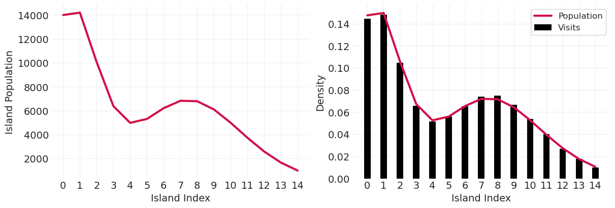
马尔可夫国王访问 Metropolis 群岛(又名 Metropolis 算法)#
抛硬币选择去左岛还是右岛
查找提议岛的人口 \(p_{proposal}\)
查找当前岛屿的人口 \(p_{current}\)
以概率 \(\frac{p_{proposal}}{p_{current}}\) 移动到提议岛屿
重复 1-4
从长远来看,此过程将访问每个岛屿,其频率与人口成正比
如果我们使用岛屿人口作为概率密度的隐喻,那么我们可以使用相同的算法,使用随机数生成器从任何概率分布(任意维度)中采样
对于贝叶斯推断,我们应用 Metropolis 算法,假设
岛屿 \(\rightarrow\) 参数值
人口规模 \(\rightarrow\) 后验概率
马尔可夫链蒙特卡洛#
链:从提议分布中抽取的一系列样本
马尔可夫链:历史无关紧要,只有参数的当前状态重要
蒙特卡洛:指在蒙特卡洛镇进行随机赌博
def simulate_markov_visits(island_sizes, n_steps=100_000):
"""aka Metropolis algorithm"""
# Metropolis algorithm
island_idx = np.arange(len(island_sizes))
visits = {ii: 0 for ii in island_idx}
current_island_idx = np.random.choice(island_idx)
markov_chain = [] # store history
for _ in range(n_steps):
# 1. Flip a coin to propose a direction, left or right
coin_flip = np.random.rand() > 0.5
direction = -1 if coin_flip else 1
proposal_island_idx = np.roll(island_idx, direction)[current_island_idx]
# 2. Proposal island size
proposal_size = island_sizes[proposal_island_idx]
# 3. Current island size
current_size = island_sizes[current_island_idx]
# 4. Go to proposal island if ratio of sizes is greater than another coin flip
p_star = proposal_size / current_size
move = np.random.rand() < p_star
current_island_idx = proposal_island_idx if move else current_island_idx
# 5. tally visits and repeat
visits[current_island_idx] += 1
markov_chain.append(current_island_idx)
# Visualization
island_idx = visits.keys()
island_visit_density = [v / n_steps for v in visits.values()]
island_size_density = island_sizes / island_sizes.sum()
_, axs = plt.subplots(1, 2, figsize=(12, 4))
plt.sca(axs[0])
plt.plot(island_sizes, lw=3, color="C0")
plt.xlabel("Island Index")
plt.ylabel("Island Population")
plt.xticks(np.arange(len(island_sizes)))
plt.sca(axs[1])
plt.plot(island_idx, island_size_density, color="C0", lw=3, label="Population")
plt.bar(island_idx, island_visit_density, color="k", width=0.4, label="Visits")
plt.xlabel("Island Index")
plt.ylabel("Density")
plt.xticks(np.arange(len(island_sizes)))
plt.legend()
return markov_chain
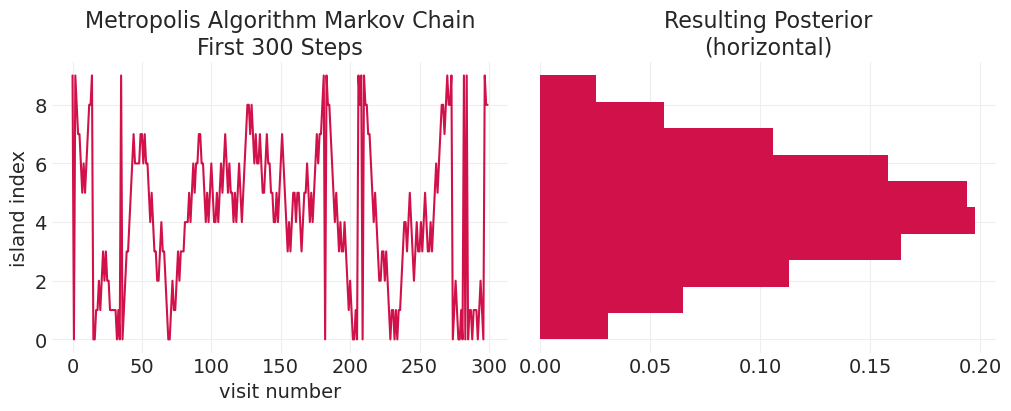
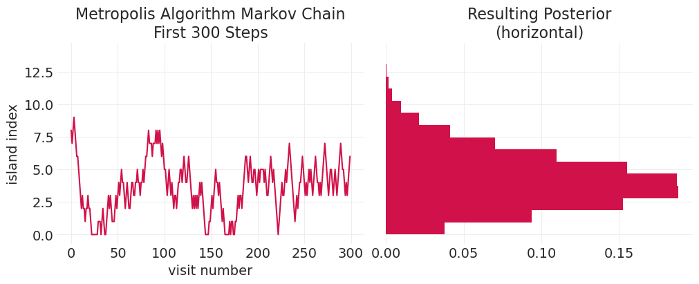
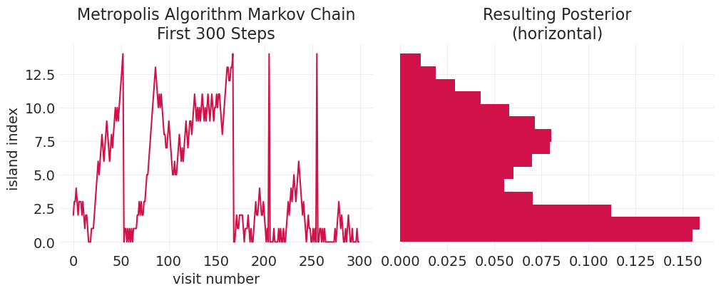
def plot_markov_chain(markov_chain, **hist_kwargs):
_, axs = plt.subplots(1, 2, figsize=(10, 4), sharey=True)
plt.sca(axs[0])
plt.plot(markov_chain[:300])
plt.xlabel("visit number")
plt.ylabel("island index")
plt.title("Metropolis Algorithm Markov Chain\nFirst 300 Steps")
plt.sca(axs[1])
plt.hist(markov_chain, orientation="horizontal", density=True, **hist_kwargs)
plt.title("Resulting Posterior\n(horizontal)");
验证算法近似于以中心岛屿为中心的高斯分布#
n_steps = 100_000
island_sizes = stats.norm(20, 10).pdf(np.linspace(1, 40, 10))
island_sizes /= island_sizes.min() / 1000

gaussian_markov_chain = simulate_markov_visits(island_sizes, n_steps)
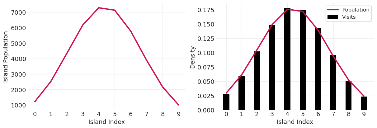
plot_markov_chain(gaussian_markov_chain, bins=10)
在泊松分布上验证#
island_sizes = stats.poisson(5).pmf(np.linspace(1, 15, 15))
island_sizes /= island_sizes.min() / 10

poisson_markov_chain = simulate_markov_visits(island_sizes, n_steps);
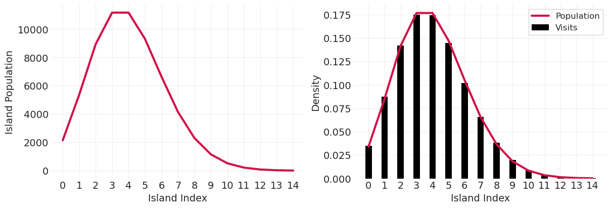
plot_markov_chain(poisson_markov_chain, bins=15)
验证更奇异的双峰分布#
island_sizes = stats.poisson(2).pmf(np.linspace(1, 15, 15)) + stats.poisson(9).pmf(
    np.linspace(1, 15, 15)
)
island_sizes /= island_sizes.min() / 1000

bimodal_markov_chain = simulate_markov_visits(island_sizes, n_steps);
plot_markov_chain(bimodal_markov_chain, bins=15)
向 Arianna Rosenbluth 致敬#
执行了原始 MCMC 算法在代码中的实际实现
在 1950 年代在 MANIAC 计算机上实现
我们可能应该称其为 Rosenbluth 算法
基本 Rosenbluth 算法#
def simulate_metropolis_algorithm(
    n_steps=100, step_size=1.0, mu=0, sigma=0.5, resolution=100, random_seed=1
):
    np.random.seed(random_seed)

    # set up parameter grid
    mu_grid = np.linspace(-3.0, 3.0, resolution)
    sigma_grid = np.linspace(0.1, 3.0, resolution)

    mus, sigmas = np.meshgrid(mu_grid, sigma_grid)
    mus = mus.ravel()
    sigmas = sigmas.ravel()

    # Distribution over actual parameters
    mu_dist = stats.norm(mu, 1)
    sigma_dist = stats.lognorm(sigma)

    # Proposal distribution for each parameter
    mu_proposal_dist = stats.norm(0, 0.25)
    sigma_proposal_dist = stats.norm(0, 0.25)

    def evaluate_log_pdf(m, s):
        log_pdf_mu = mu_dist.logpdf(m)
        log_pdf_sigma = sigma_dist.logpdf(s)
        return log_pdf_mu + log_pdf_sigma

    def calculate_acceptance_probability(current_mu, current_sigma, proposal_mu, proposal_sigma):
        current_log_prob = evaluate_log_pdf(current_mu, current_sigma)
        proposal_log_prob = evaluate_log_pdf(proposal_mu, proposal_sigma)

        return np.exp(np.min([0, proposal_log_prob - current_log_prob]))

    # Contour plot of the joint distribution over parameters
    log_pdf_mu = mu_dist.logpdf(mus)
    log_pdf_sigma = sigma_dist.logpdf(sigmas)

    joint_log_pdf = log_pdf_mu + log_pdf_sigma
    joint_pdf = np.exp(joint_log_pdf - joint_log_pdf.max())

    plt.contour(
        mus.reshape(resolution, resolution),
        np.log(sigmas).reshape(resolution, resolution),
        joint_pdf.reshape(resolution, resolution),
        cmap="gray_r",
    )

    # Run the Metropolis algorithm
    current_mu = np.random.choice(mus)
    current_sigma = np.random.choice(sigmas)

    accept_count = 0
    reject_count = 0
    for step in range(n_steps):

        # Propose a new location in parameter space nearby to the current params
        proposal_mu = current_mu + mu_proposal_dist.rvs() * step_size
        proposal_sigma = current_sigma + sigma_proposal_dist.rvs() * step_size

        # Accept proposal?
        acceptance_prob = calculate_acceptance_probability(
            current_mu, current_sigma, proposal_mu, proposal_sigma
        )
        if acceptance_prob >= np.random.rand():
            accept_label = "accepted" if accept_count == 0 else None
            plt.scatter(
                (current_mu, proposal_mu),
                (np.log(current_sigma), np.log(proposal_sigma)),
                color="C0",
                alpha=0.25,
                label=accept_label,
            )
            plt.plot(
                (current_mu, proposal_mu),
                (np.log(current_sigma), np.log(proposal_sigma)),
                color="C0",
                alpha=0.25,
            )
            current_mu = proposal_mu
            current_sigma = proposal_sigma
            accept_count += 1
        else:
            reject_label = "rejected" if reject_count == 0 else None
            plt.scatter(
                (current_mu, proposal_mu),
                (np.log(current_sigma), np.log(proposal_sigma)),
                color="black",
                alpha=1,
                label=reject_label,
            )
            reject_count += 1

    accept_rate = accept_count / n_steps

    plt.xlabel(r"$\mu$")
    plt.ylabel(r"$log \; \sigma$")
    plt.xlim([mus.min(), mus.max()])
    plt.ylim([np.log(sigmas.min()), np.log(sigmas.max())])
    plt.title(f"step size: {step_size}; accept rate: {accept_rate}")
    plt.legend()
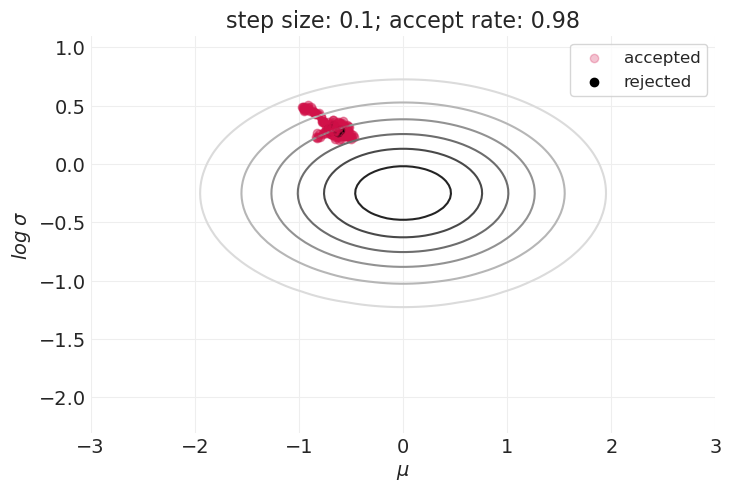
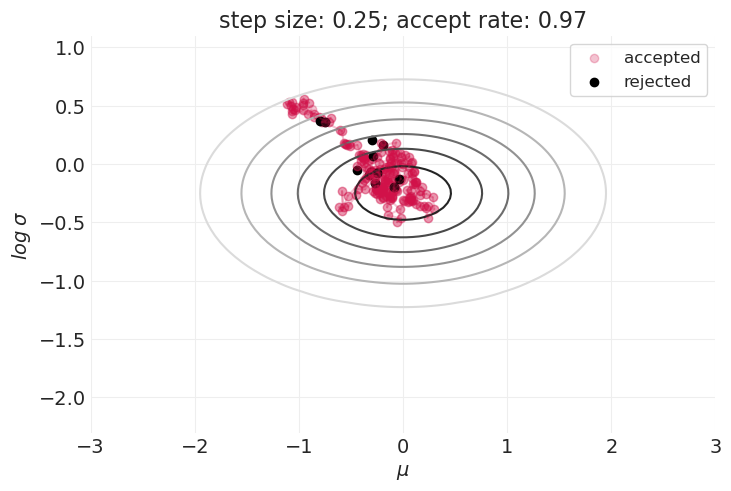
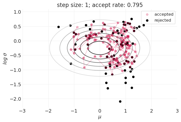
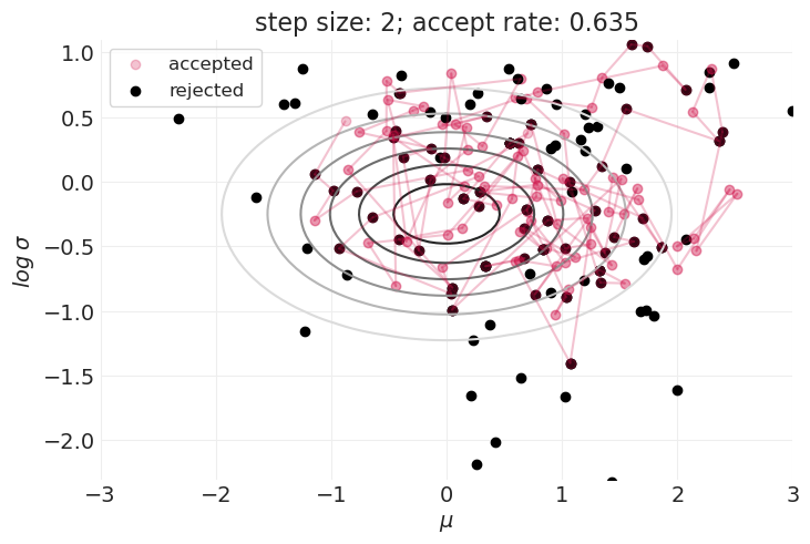
步长的影响#
for step_size in [0.1, 0.25, 0.5, 1, 2]:
    plt.figure()
    simulate_metropolis_algorithm(step_size=step_size, n_steps=200)

Metropolis 算法非常棒,因为它#
非常简单
通用 – 它可以应用于任何分布
但是,它也有一些主要的缺点#
如上所示,在探索分布的形状和接受样本之间存在权衡。
这在具有更高维度参数空间的模型中只会变得更糟。
样本的大拒绝率可能会使 Metropolis 算法在实践中无法使用。
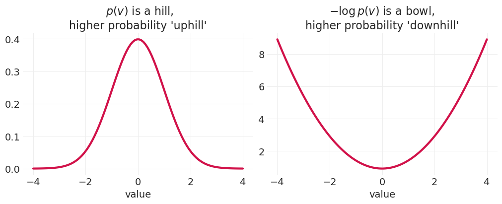
哈密顿又名“混合”蒙特卡洛 (HMC) 🛹#
HMC 是一种更有效的采样算法,它利用关于后验的梯度信息,以提高采样效率——探索更多的空间,同时接受更多提议的样本。它通过将参数空间中的每个位置与物理模拟空间中的位置相关联来实现这一点。然后,我们使用哈密顿动力学运行物理模拟,哈密顿动力学以在表面上移动的粒子的位置和动量来表示。在表面上的任何点,粒子都将具有势能 U 和动能 K,由于能量守恒,它们会来回交换。HMC 使用这种能量守恒来模拟动力学。
demo_posterior = stats.norm
values = np.linspace(-4, 4, 100)
pdf = demo_posterior.pdf(values)
neg_log_pdf = -demo_posterior.logpdf(values)
_, axs = plt.subplots(1, 2, figsize=(10, 4))
plt.sca(axs[0])
utils.plot_line(values, pdf, label="PDF")
plt.xlabel("value")
plt.title("$\\ p(v)$ is a hill,\nhigher probability 'uphill'")

plt.sca(axs[1])
utils.plot_line(values, neg_log_pdf, label="PDF")
plt.xlabel("value")
plt.title("$-\\log p(v)$ is a bowl,\nhigher probability 'downhill'");
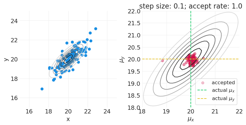
HMC 需要几个组件:#
一个函数
U(position),它从物理动力学的角度返回“势能”。这与给定数据和当前参数的负对数后验相同。U(position)的梯度,dU(position),它提供关于势能/参数的偏导数,给定数据样本和当前参数状态。一个函数
K(momentum),它返回给定模拟粒子当前动量的势能。
有关更多详细信息,请参阅我的(现在很久以前的)关于 MCMC 的博客文章:哈密顿蒙特卡洛
from functools import partial


def U_(x, y, theta, a=0, b=1, c=0, d=1):
    """
    Potential energy / negative log-posterior given current parameters, theta.
    a, b and c, d are the mean and variance of prior distributions for mu_x and
    mu_y, respectively
    """
    mu_x, mu_y = theta

    # Gaussian log priors
    log_prior_mu_x = stats.norm(a, b).logpdf(mu_x)
    log_prior_mu_y = stats.norm(c, d).logpdf(mu_y)

    # Gaussian log likelihoods
    log_likelihood_x = np.sum(stats.norm(mu_x, 1).logpdf(x))
    log_likelihood_y = np.sum(stats.norm(mu_y, 1).logpdf(y))

    # log posterior
    log_posterior = log_likelihood_x + log_likelihood_y + log_prior_mu_x + log_prior_mu_y

    # potential energy is negative log posterior
    return -log_posterior


def dU_(x, y, theta, a=0, b=1, c=0, d=1):
    """
    Gradient of potential energy with respect to current parameters, theta.
    a, b and c, d are the mean and variance of prior distributions for mu_x and
    mu_y, respectively
    """
    mu_x, mu_y = theta

    # Note: we implicitly divide by likelihood (left) term
    # of the gradient by the likelihood variance, which is 1
    dU_dmu_x = np.sum(x - mu_x) + (a - mu_x) / b**2
    dU_dmu_y = np.sum(y - mu_y) + (c - mu_y) / d**2
    return np.array((-dU_dmu_x, -dU_dmu_y))


def K(momentum):
    """Kinetic energy given a current momentum state"""
    return np.sum(momentum**2) / 2
HMC 的每个步骤都涉及“轻弹”粒子,使其具有特定的动量(速度和方向),然后允许粒子在能量景观表面上“滚动”。粒子在任何时间点所采取的方向由函数 dU() 给出。为了模拟沿景观的非线性运动,我们采取多个连续的线性步骤(又名“蛙跳”步骤)。在采取一定数量的步骤后,我们计算系统的总能量,这是势能(由 U() 给出)和动能的组合,动能可以直接从动量状态计算出来。如果模拟后的势能状态(负对数后验)低于初始状态(动力学之前)的势能,那么我们根据能量变化随机接受参数的新状态。
def HMC(current_theta, U, dU, step_size, n_leapfrog_steps):
    """Propose/accept a parameter sample using Hamiltonian / Hybrid Monte Carlo"""
    n_parameters = len(current_theta)

    # Initial "position" and "momentum"
    position = current_theta
    momentum = stats.norm().rvs(n_parameters)  # random flick

    current_momentum = momentum

    # Take a half step at beginning
    momentum -= (step_size / 2) * dU(theta=position)

    # Simulate nonlinear dynamics with linear leapfrog steps
    for step in range(n_leapfrog_steps - 1):
        position += step_size * momentum
        momentum -= step_size * dU(theta=position)

    # Take half step at the end
    momentum -= (step_size / 2) * dU(theta=position)

    # Negate momentum at end for symmetric proposal
    momentum *= -1

    # Calculate potential/kinetic energies at beginning / end of simulation
    current_U = U(theta=current_theta)
    current_K = K(current_momentum)

    proposed_U = U(theta=position)
    proposed_K = K(momentum)

    # Acceptance criterion
    acceptance_probability = np.exp(
        np.min([0, (current_U - proposed_U) + (current_K - proposed_K)])
    )
    if acceptance_probability > np.random.rand():
        new_theta = position
        accept = 1
    else:
        new_theta = current_theta
        accept = 0

    return new_theta, accept


def simulate_hybrid_monte_carlo(
    mu=np.array((20, 10)),
    covariance=np.eye(2),
    n_samples=10,
    n_steps=100,
    step_size=0.01,
    n_leapfrog_steps=11,
    resolution=100,
    random_seed=123,
):
    """
    Simulate running HMC sampler to estimate the parameters mu = (mu_x and mu_y).
    """
    np.random.seed(random_seed)

    # The true data distribution
    data_dist = stats.multivariate_normal(mu, covariance)

    # Sample data points from the true distribution -- this will guide the posterior
    dataset = data_dist.rvs(n_samples).T
    x = dataset[0]
    y = dataset[1]

    # Parameter grid for visualization
    mux, muy = mu[0], mu[1]
    mux_grid = np.linspace(mux - mux * 0.25, mux + mux * 0.25, resolution)
    muy_grid = np.linspace(muy - muy * 0.25, muy + muy * 0.25, resolution)

    xs, ys = np.meshgrid(mux_grid, muy_grid)
    xs = xs.ravel()
    ys = ys.ravel()

    # Plot the true data distribution and samples
    true_pdf = data_dist.pdf(np.vstack([xs, ys]).T)
    _, axs = plt.subplots(1, 2, figsize=(8, 4))
    plt.sca(axs[0])
    plt.contour(
        xs.reshape(resolution, resolution),
        ys.reshape(resolution, resolution),
        true_pdf.reshape(resolution, resolution),
        cmap="gray_r",
    )
    plt.scatter(x, y, color="C1", label="data")

    plt.xlim([xs.min(), xs.max()])
    plt.ylim([ys.min(), ys.max()])
    plt.xlabel("x")
    plt.ylabel("y")

    # Display HMC dynamics
    plt.sca(axs[1])

    # Add true pdf to dynamics plot
    plt.contour(
        xs.reshape(resolution, resolution),
        ys.reshape(resolution, resolution),
        true_pdf.reshape(resolution, resolution),
        cmap="gray_r",
    )

    # Initialize the potential energy and gradient functions with the data points
    U = partial(U_, x=x, y=y)
    dU = partial(dU_, x=x, y=y)

    # Use datapoint as random starting point
    current_theta = np.array((np.random.choice(x), np.random.choice(y)))
    accept_count = 0
    reject_count = 0
    for step in range(n_steps):

        # Run Hybrid Monte Carlo Step
        proposed_theta, accept = HMC(current_theta, U, dU, step_size, n_leapfrog_steps)

        # Plot sampling progress
        if accept:
            accept_label = "accepted" if accept_count == 0 else None

            plt.scatter(
                (current_theta[0], proposed_theta[0]),
                (current_theta[1], proposed_theta[1]),
                color="C0",
                alpha=0.25,
                label=accept_label,
            )
            plt.plot(
                (current_theta[0], proposed_theta[0]),
                (current_theta[1], proposed_theta[1]),
                color="C0",
                alpha=0.25,
            )
            current_theta = proposed_theta
            accept_count += 1
        else:
            reject_label = "rejected" if reject_count == 0 else None
            plt.scatter(
                proposed_theta[0], proposed_theta[1], color="black", alpha=0.25, label=reject_label
            )
            reject_count += 1

    accept_rate = accept_count / n_steps

    # Show true parameters
    plt.axvline(mux, linestyle="--", color="C2", label="actual $\\mu_x$")
    plt.axhline(muy, linestyle="--", color="C3", label="actual $\\mu_y$")

    # Style
    plt.xlim([mux - mux * 0.1, mux + mux * 0.1])
    plt.ylim([muy - muy * 0.1, muy + muy * 0.1])
    plt.xlabel("$\\mu_x$")
    plt.ylabel("$\\mu_y$")
    plt.title(f"step size: {step_size}; accept rate: {accept_rate}")
    plt.legend(loc="lower right")
微积分是超能力#
自动微分#
对于上面的 HMC 示例,我们的(对数)后验/势能具有特定的函数形式(即多维高斯分布),并且我们必须使用特定的梯度和代码来计算与该后验对齐的那些梯度。这种自定义的推断方法通常是不可行的,因为
计算关于每个参数的梯度需要大量工作
您必须为每个模型重新编码(和调试)算法
自动微分允许我们使用任何后验函数,从而免费为我们提供梯度。基本上,该函数被分解为最基本的数学运算的计算链。每个基本运算都有其自身的简单导数,因此我们可以将这些导数链接在一起,以自动提供整个函数关于任何参数的梯度。
Stan / PyMC#
McElreath 使用 Stan(通过 R 访问)来访问自动微分并运行一般贝叶斯推断。我们使用 PyMC,一种类似的概率编程语言 (PPL)。
2012 年新泽西州葡萄酒品鉴会#
20 种葡萄酒
10 种法国葡萄酒,10 种新泽西州葡萄酒
9 位法国 & 美国评委
总共 180 个评分
葡萄酒
100 种新泽西州
80 种法国
评委
108 位新泽西州
72 位法国
WINES = utils.load_data("Wines2012")
WINES.head()
| 评委 | 轮次 | 葡萄酒 | 评分 | wine.amer | judge.amer | |
|---|---|---|---|---|---|---|
| 0 | Jean-M Cardebat | 白色 | A1 | 10.0 | 1 | 0 |
| 1 | Jean-M Cardebat | 白色 | B1 | 13.0 | 1 | 0 |
| 2 | Jean-M Cardebat | 白色 | C1 | 14.0 | 0 | 0 |
| 3 | Jean-M Cardebat | 白色 | D1 | 15.0 | 0 | 0 |
| 4 | Jean-M Cardebat | 白色 | E1 | 8.0 | 1 | 0 |
utils.draw_causal_graph(
    edge_list=[("Q", "S"), ("X", "Q"), ("X", "S"), ("J", "S"), ("Z", "J")],
    node_props={
        "Q": {"label": "Wine Quality, Q", "style": "dashed", "color": "red"},
        "J": {"label": "Judge Behavior, J", "style": "dashed"},
        "X": {"label": "Wine Origin, X", "color": "red"},
        "S": {"label": "Wine Score, S"},
        "Z": {"label": "Judge Origin, Z"},
        "unobserved": {"style": "dashed"},
    },
    edge_props={("X", "S"): {"style": "dashed"}, ("X", "Q"): {"color": "red"}},
)

估计量#
葡萄酒质量和葡萄酒产地之间的关联
按评委分层(不是必需的)以提高效率
最简单的模型#
确保从简单开始
请注意,质量 \(Q_{W_[i]}\) 是一个未观察到的潜在变量。
# Define & preprocess data / coords

# Continuous, standardized wine scores
SCORES = utils.standardize(WINES.score).values

# Categorical judge ID
JUDGE_ID, JUDGE = pd.factorize(WINES.judge)

# Categorical wine ID
WINE_ID, WINE = pd.factorize(WINES.wine)

# Categorical wine origin
WINE_ORIGIN_ID, WINE_ORIGIN = pd.factorize(
    ["US" if w == 1.0 else "FR" for w in WINES["wine.amer"]], sort=False
)
拟合简单的、特定于葡萄酒的模型#
with pm.Model(coords={"wine": WINE}) as simple_model:

    sigma = pm.Exponential("sigma", 1)
    Q = pm.Normal("Q", 0, 1, dims="wine")  # Wine ID
    mu = Q[WINE_ID]
    S = pm.Normal("S", mu, sigma, observed=SCORES)
    simple_inference = pm.sample()
Initializing NUTS using jitter+adapt_diag...
Multiprocess sampling (4 chains in 4 jobs)
NUTS: [sigma, Q]
Sampling 4 chains for 1_000 tune and 1_000 draw iterations (4_000 + 4_000 draws total) took 1 seconds.
后验摘要#
az.summary(simple_inference)
| 均值 | 标准差 | hdi_3% | hdi_97% | mcse_mean | mcse_sd | ess_bulk | ess_tail | r_hat | |
|---|---|---|---|---|---|---|---|---|---|
| Q[A1] | 0.135 | 0.329 | -0.447 | 0.778 | 0.003 | 0.005 | 11039.0 | 2969.0 | 1.00 |
| Q[B1] | 0.274 | 0.328 | -0.369 | 0.875 | 0.003 | 0.004 | 9868.0 | 2969.0 | 1.00 |
| Q[C1] | -0.121 | 0.319 | -0.704 | 0.474 | 0.003 | 0.005 | 9702.0 | 2878.0 | 1.00 |
| Q[D1] | 0.292 | 0.321 | -0.292 | 0.896 | 0.004 | 0.004 | 8275.0 | 2700.0 | 1.00 |
| Q[E1] | 0.085 | 0.321 | -0.521 | 0.695 | 0.003 | 0.006 | 10652.0 | 2742.0 | 1.01 |
| Q[F1] | -0.013 | 0.317 | -0.606 | 0.583 | 0.003 | 0.006 | 10452.0 | 2963.0 | 1.00 |
| Q[G1] | -0.110 | 0.307 | -0.648 | 0.489 | 0.003 | 0.005 | 9953.0 | 3314.0 | 1.00 |
| Q[H1] | -0.218 | 0.316 | -0.824 | 0.347 | 0.004 | 0.004 | 7694.0 | 2506.0 | 1.00 |
| Q[I1] | -0.144 | 0.329 | -0.743 | 0.481 | 0.003 | 0.005 | 9632.0 | 2801.0 | 1.00 |
| Q[J1] | -0.162 | 0.322 | -0.776 | 0.435 | 0.003 | 0.005 | 9654.0 | 2855.0 | 1.00 |
| Q[A2] | 0.104 | 0.309 | -0.455 | 0.701 | 0.003 | 0.005 | 8660.0 | 3420.0 | 1.00 |
| Q[B2] | 0.561 | 0.312 | -0.047 | 1.112 | 0.003 | 0.003 | 11413.0 | 3002.0 | 1.00 |
| Q[C2] | -0.371 | 0.311 | -0.944 | 0.222 | 0.003 | 0.003 | 12525.0 | 2978.0 | 1.00 |
| Q[D2] | 0.271 | 0.315 | -0.340 | 0.829 | 0.003 | 0.004 | 8610.0 | 3113.0 | 1.00 |
| Q[E2] | 0.121 | 0.326 | -0.478 | 0.734 | 0.003 | 0.005 | 10737.0 | 2991.0 | 1.00 |
| Q[F2] | -0.030 | 0.315 | -0.596 | 0.579 | 0.003 | 0.006 | 9762.0 | 2874.0 | 1.00 |
| Q[G2] | 0.008 | 0.323 | -0.608 | 0.599 | 0.003 | 0.006 | 10383.0 | 2651.0 | 1.00 |
| Q[H2] | -0.198 | 0.318 | -0.791 | 0.384 | 0.003 | 0.005 | 10027.0 | 2909.0 | 1.00 |
| Q[I2] | -0.856 | 0.328 | -1.504 | -0.277 | 0.003 | 0.003 | 10050.0 | 2731.0 | 1.00 |
| Q[J2] | 0.387 | 0.318 | -0.199 | 1.014 | 0.003 | 0.004 | 9533.0 | 2864.0 | 1.00 |
| sigma | 1.000 | 0.054 | 0.905 | 1.110 | 0.001 | 0.000 | 6766.0 | 2798.0 | 1.00 |
az.plot_forest(simple_inference, combined=True);
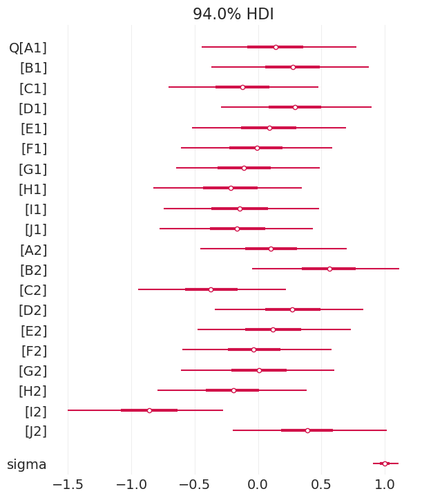
绘制马尔可夫猫头鹰 🦉#
收敛性评估#
迹图
迹秩图
R-hat 收敛性度量
n_effective 样本
发散跃迁
1. 迹图#
寻找
“模糊的毛毛虫”
“游荡”路径表示步长太小(接受次数多,但仅探索局部空间)
相同值的长时间段表示步长太大(拒绝次数多,未探索空间)
每个参数应在链中具有相似的密度
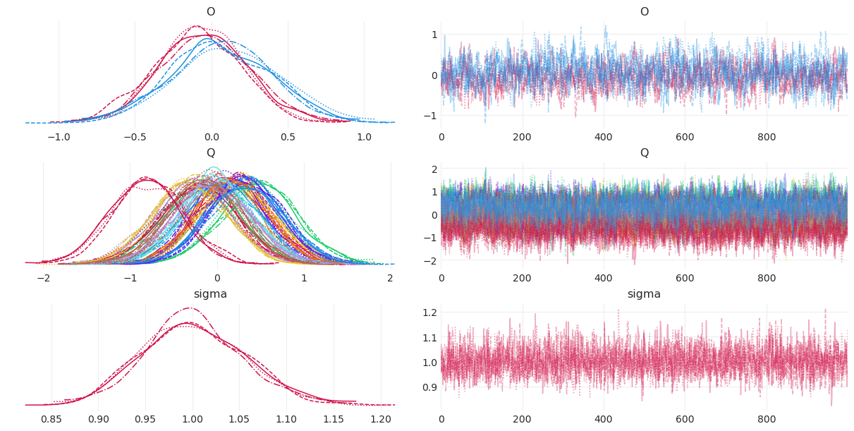
单独查看所有参数#
az.plot_trace(simple_inference, compact=False, legend=True);
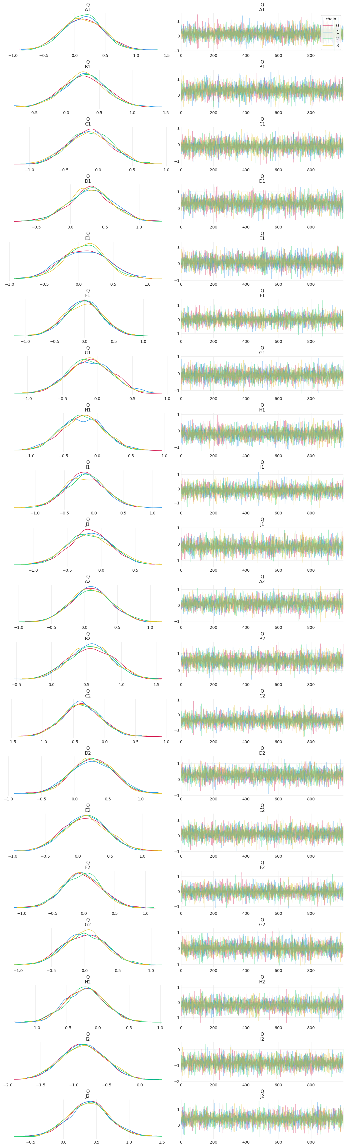
这么多模糊的毛毛虫!
如果 HMC 采样正确,您只需要几百个样本即可很好地了解后验的形状。这是因为,在正确的初始条件和模型参数化下,HMC 非常有效。
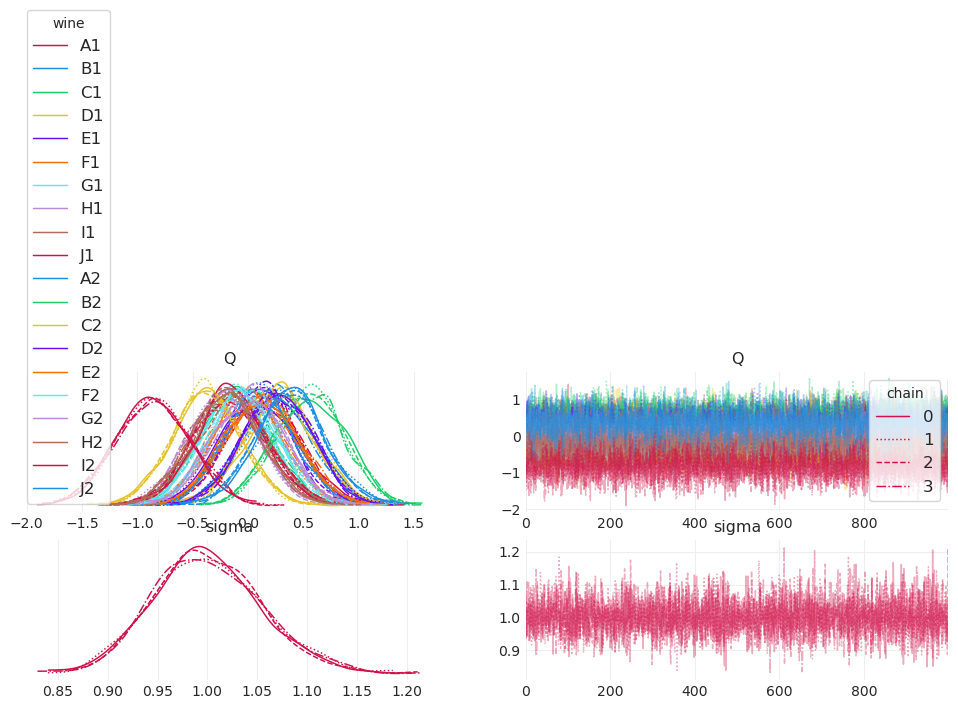
信息量很大!尝试紧凑形式#
az.plot_trace(simple_inference, compact=True, legend=True);
2. 迹秩“Trank”图#
不希望任何一条链长时间具有最大或最小秩。
“混乱”是好的
az.plot_rank(simple_inference);
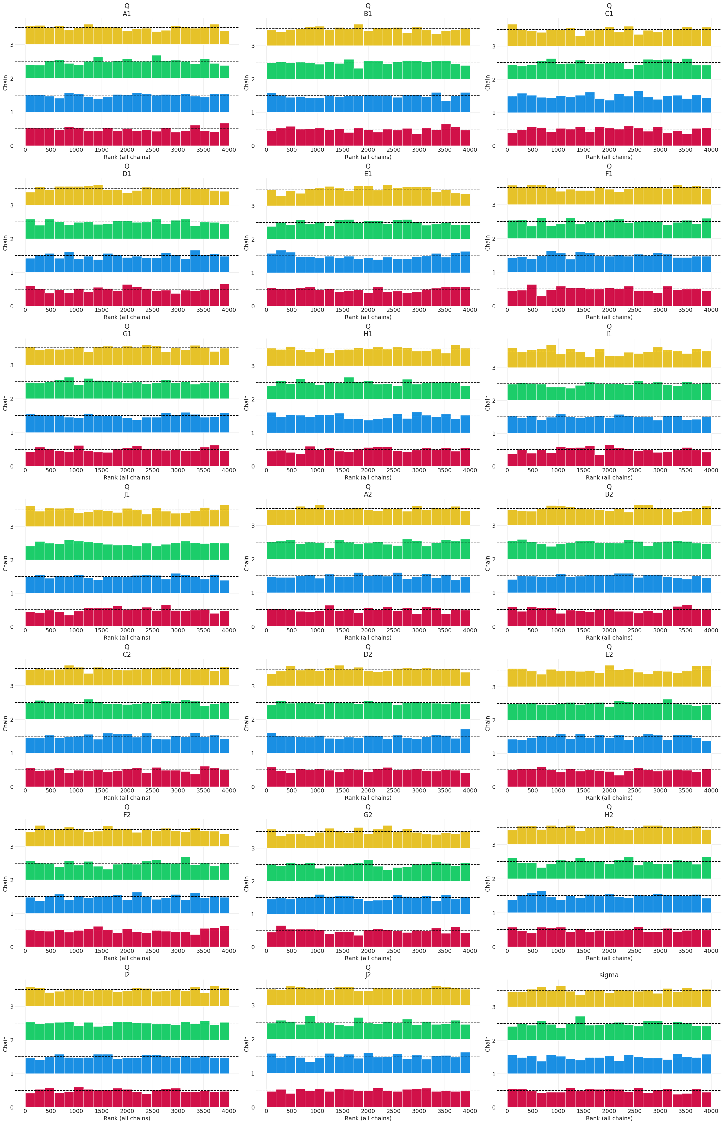
与每条链相关的Trank图都围绕平均值(虚线)盘旋,这表明一组混合良好、高效的马尔可夫链。
3. R-hat#
链收敛性度量
比较链内方差与链间方差的方差比率
类似于用于训练 k-means 的指标(相反)
想法是,如果链已收敛并且正在探索相同的空间,那么它们的链内方差应与链间方差或多或少相同,从而提供接近 1.0 的 R-hat。
不保证。这不是测试。
没有神奇的值;但要注意 1.1 左右或更高的值 🤷♂️
4. 有效样本大小 (ESS)#
存在
ess_*,其中tail和bulk是估计有效样本的不同方法tail似乎给出了 burnin 后的 ESS 样本想法是估计可用的样本数量,这些样本彼此之间接近独立
往往小于实际运行的样本数量(因为实际样本在现实世界中实际上不是独立的)
显示诊断信息#
az.summary(simple_inference)[["ess_bulk", "ess_tail", "r_hat"]]
| ess_bulk | ess_tail | r_hat | |
|---|---|---|---|
| Q[A1] | 11039.0 | 2969.0 | 1.00 |
| Q[B1] | 9868.0 | 2969.0 | 1.00 |
| Q[C1] | 9702.0 | 2878.0 | 1.00 |
| Q[D1] | 8275.0 | 2700.0 | 1.00 |
| Q[E1] | 10652.0 | 2742.0 | 1.01 |
| Q[F1] | 10452.0 | 2963.0 | 1.00 |
| Q[G1] | 9953.0 | 3314.0 | 1.00 |
| Q[H1] | 7694.0 | 2506.0 | 1.00 |
| Q[I1] | 9632.0 | 2801.0 | 1.00 |
| Q[J1] | 9654.0 | 2855.0 | 1.00 |
| Q[A2] | 8660.0 | 3420.0 | 1.00 |
| Q[B2] | 11413.0 | 3002.0 | 1.00 |
| Q[C2] | 12525.0 | 2978.0 | 1.00 |
| Q[D2] | 8610.0 | 3113.0 | 1.00 |
| Q[E2] | 10737.0 | 2991.0 | 1.00 |
| Q[F2] | 9762.0 | 2874.0 | 1.00 |
| Q[G2] | 10383.0 | 2651.0 | 1.00 |
| Q[H2] | 10027.0 | 2909.0 | 1.00 |
| Q[I2] | 10050.0 | 2731.0 | 1.00 |
| Q[J2] | 9533.0 | 2864.0 | 1.00 |
| sigma | 6766.0 | 2798.0 | 1.00 |
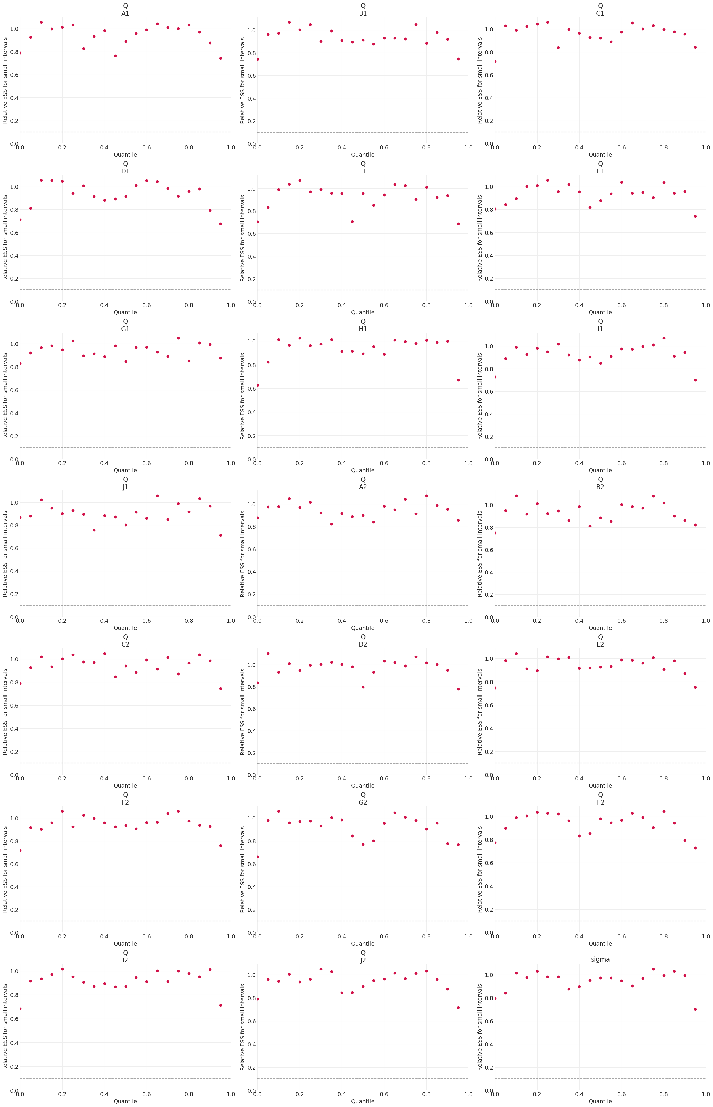
ESS 图#
局部 ESS 图#
局部 ESS 越高越好,表明马尔可夫链更有效
高效的马尔可夫链应展示相对 ESS 值
az.plot_ess(simple_inference, kind="local", relative=True);
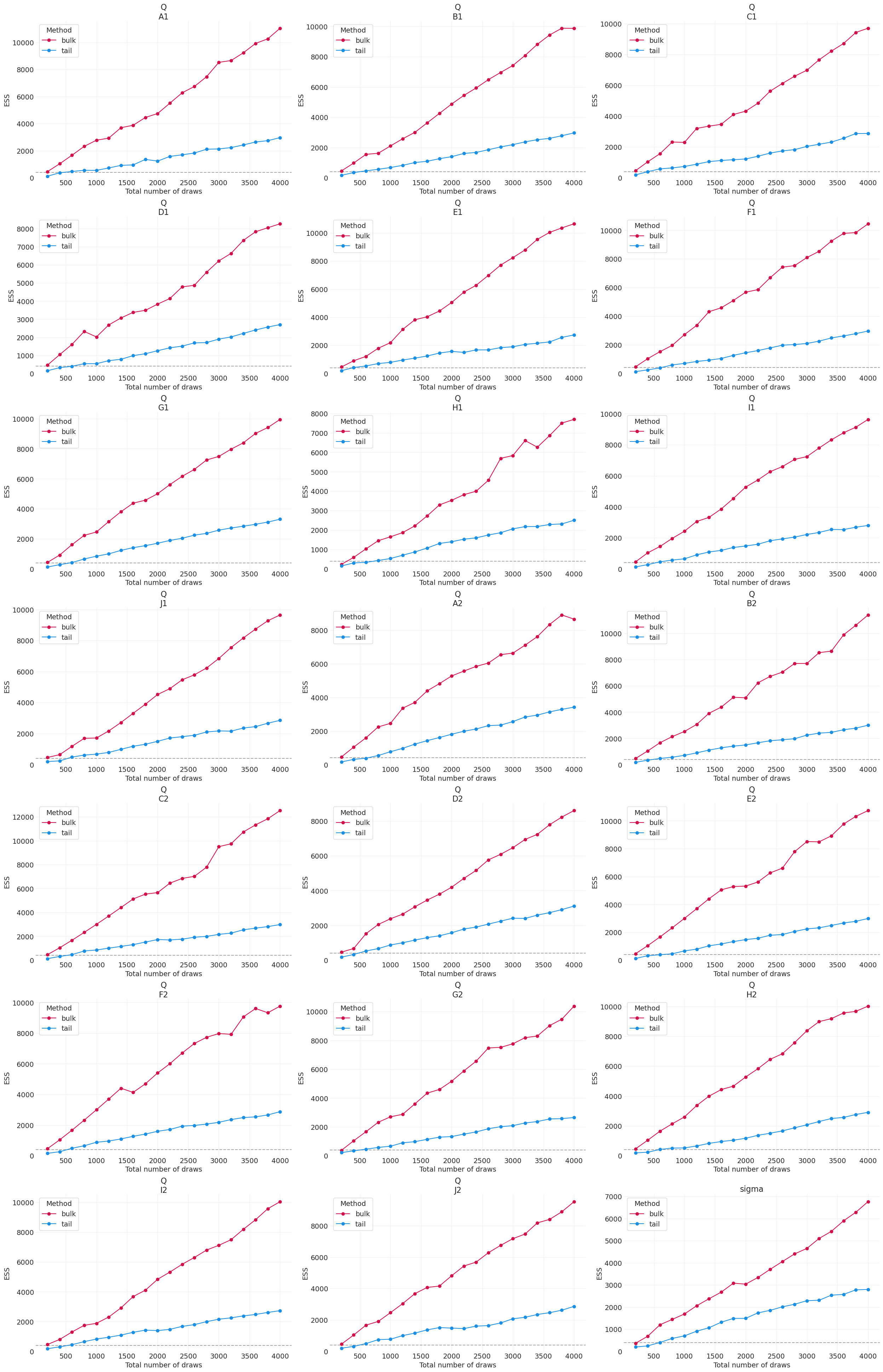
ESS 演化图#
对于正在收敛的马尔可夫链,ESS 应随着链中抽取的数量持续增加
对于
bulk和tail,ESS 与抽取次数应大致呈线性关系
az.plot_ess(simple_inference, kind="evolution");
更完整的模型,按葡萄酒产地分层,\(O_{X[i]}\)#
拟合葡萄酒产地模型#
with pm.Model(coords={"wine": WINE, "wine_origin": WINE_ORIGIN}) as wine_origin_model:
    sigma = pm.Exponential("sigma", 1)
    O = pm.Normal("O", 0, 1, dims="wine_origin")  # Wine Origin
    Q = pm.Normal("Q", 0, 1, dims="wine")  # Wine ID
    mu = Q[WINE_ID] + O[WINE_ORIGIN_ID]
    S = pm.Normal("S", mu, sigma, observed=SCORES)

    wine_origin_inference = pm.sample()
Initializing NUTS using jitter+adapt_diag...
Multiprocess sampling (4 chains in 4 jobs)
NUTS: [sigma, O, Q]
Sampling 4 chains for 1_000 tune and 1_000 draw iterations (4_000 + 4_000 draws total) took 1 seconds.
MCMC 诊断#
az.plot_trace(wine_origin_inference, compact=True);
后验摘要#
az.summary(wine_origin_inference)
| 均值 | 标准差 | hdi_3% | hdi_97% | mcse_mean | mcse_sd | ess_bulk | ess_tail | r_hat | |
|---|---|---|---|---|---|---|---|---|---|
| O[US] | -0.061 | 0.290 | -0.575 | 0.532 | 0.011 | 0.008 | 706.0 | 1243.0 | 1.01 |
| O[FR] | 0.073 | 0.341 | -0.538 | 0.747 | 0.012 | 0.008 | 824.0 | 1351.0 | 1.01 |
| Q[A1] | 0.193 | 0.407 | -0.561 | 0.966 | 0.012 | 0.008 | 1205.0 | 2143.0 | 1.00 |
| Q[B1] | 0.325 | 0.402 | -0.415 | 1.098 | 0.012 | 0.008 | 1156.0 | 1632.0 | 1.01 |
| Q[C1] | -0.192 | 0.450 | -1.074 | 0.589 | 0.012 | 0.009 | 1348.0 | 2292.0 | 1.01 |
| Q[D1] | 0.224 | 0.448 | -0.618 | 1.061 | 0.012 | 0.008 | 1428.0 | 2107.0 | 1.00 |
| Q[E1] | 0.143 | 0.398 | -0.567 | 0.915 | 0.011 | 0.008 | 1291.0 | 2448.0 | 1.00 |
| Q[F1] | 0.036 | 0.418 | -0.756 | 0.803 | 0.011 | 0.008 | 1329.0 | 2380.0 | 1.00 |
| Q[G1] | -0.052 | 0.418 | -0.844 | 0.691 | 0.011 | 0.008 | 1440.0 | 2525.0 | 1.00 |
| Q[H1] | -0.287 | 0.439 | -1.114 | 0.543 | 0.012 | 0.009 | 1250.0 | 2166.0 | 1.00 |
| Q[I1] | -0.086 | 0.414 | -0.876 | 0.677 | 0.012 | 0.008 | 1229.0 | 1955.0 | 1.00 |
| Q[J1] | -0.229 | 0.447 | -1.140 | 0.555 | 0.013 | 0.009 | 1242.0 | 2007.0 | 1.01 |
| Q[A2] | 0.043 | 0.437 | -0.816 | 0.843 | 0.013 | 0.009 | 1200.0 | 2190.0 | 1.01 |
| Q[B2] | 0.484 | 0.443 | -0.350 | 1.326 | 0.012 | 0.009 | 1360.0 | 2206.0 | 1.00 |
| Q[C2] | -0.309 | 0.416 | -1.072 | 0.472 | 0.011 | 0.008 | 1386.0 | 2037.0 | 1.00 |
| Q[D2] | 0.328 | 0.413 | -0.532 | 1.038 | 0.011 | 0.008 | 1310.0 | 1719.0 | 1.00 |
| Q[E2] | 0.179 | 0.403 | -0.548 | 0.958 | 0.011 | 0.008 | 1342.0 | 2241.0 | 1.01 |
| Q[F2] | 0.022 | 0.408 | -0.741 | 0.777 | 0.011 | 0.008 | 1352.0 | 1914.0 | 1.00 |
| Q[G2] | -0.052 | 0.443 | -0.894 | 0.768 | 0.012 | 0.009 | 1286.0 | 1871.0 | 1.01 |
| Q[H2] | -0.144 | 0.408 | -0.857 | 0.650 | 0.011 | 0.008 | 1275.0 | 1855.0 | 1.00 |
| Q[I2] | -0.808 | 0.412 | -1.587 | -0.038 | 0.011 | 0.008 | 1314.0 | 2414.0 | 1.00 |
| Q[J2] | 0.320 | 0.446 | -0.516 | 1.153 | 0.012 | 0.008 | 1390.0 | 2342.0 | 1.00 |
| sigma | 1.002 | 0.055 | 0.902 | 1.103 | 0.001 | 0.001 | 2914.0 | 3001.0 | 1.00 |
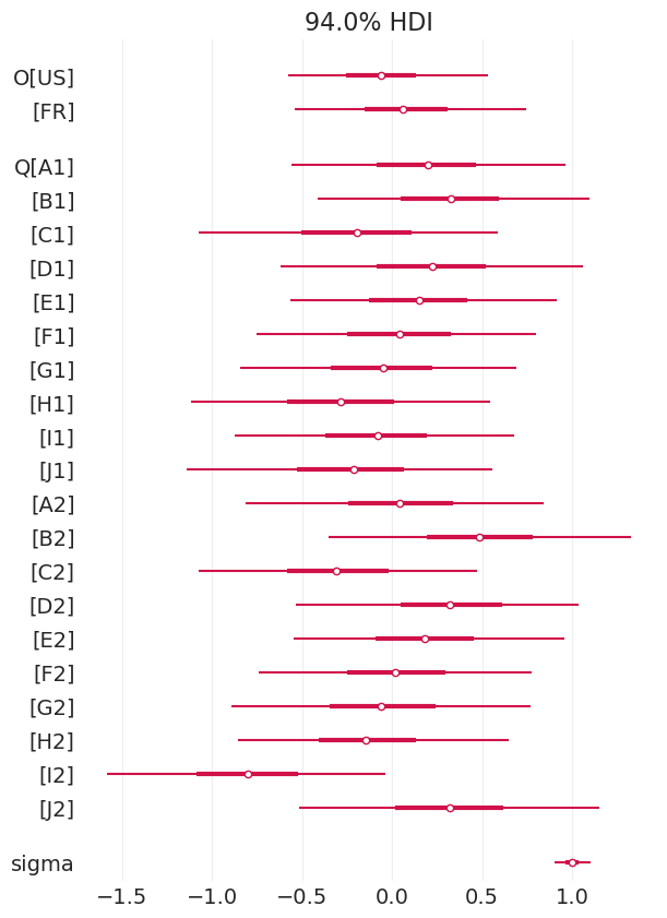
az.plot_forest(wine_origin_inference, combined=True);
包括评委效应#
utils.draw_causal_graph(
    edge_list=[("Q", "S"), ("X", "Q"), ("X", "S"), ("J", "S"), ("Z", "J")],
    node_props={
        "Q": {"color": "red"},
        "J": {"style": "dashed"},
        "X": {"color": "red"},
        "unobserved": {"style": "dashed"},
    },
    edge_props={("X", "S"): {"style": "dashed"}, ("X", "Q"): {"color": "red"}},
)

查看 DAG(上方),我们看到评委的区分是衡量分数的竞争原因。
我们使用项目反应型模型来包含评委效应,用于平均分数:\(\mu_i = (Q_{W[i]} + O_{X[i]} - H_{J[i]})D_{J[i]}\)
其中分数 \(S_i\) 的均值 \(\mu_i\) 建模为以下项的线性组合
葡萄酒质量 \(Q_{W[i]}\)
葡萄酒产地 \(O_{X[i[}\)
评委的基线评分严格程度 \(H_{J[i]}\)
值 \(< 0\) 表示评委不太可能像平均水平那样对葡萄酒给出差评
所有这些都由评委的区分能力 \(D_{J[i]}\) 调节(相乘)
值 \(> 1\) 表示评委为葡萄酒差异提供更大的分数差异
值 \(< 1\) 表示评委为葡萄酒差异提供较小的分数差异
值为 0 表示评委给所有葡萄酒一个平均分数
统计模型#
拟合评委模型#
with pm.Model(coords={"wine": WINE, "wine_origin": WINE_ORIGIN, "judge": JUDGE}) as judges_model:

    # Judge effects
    D = pm.Exponential("D", 1, dims="judge")  # Judge Discrimination (multiplicative)
    H = pm.Normal("H", 0, 1, dims="judge")  # Judge Harshness (additive)

    # Wine Origin effect
    O = pm.Normal("O", 0, 1, dims="wine_origin")

    # Wine Quality effect
    Q = pm.Normal("Q", 0, 1, dims="wine")

    # Score
    sigma = pm.Exponential("sigma", 1)

    # Likelihood
    mu = (O[WINE_ORIGIN_ID] + Q[WINE_ID] - H[JUDGE_ID]) * D[JUDGE_ID]
    S = pm.Normal("S", mu, sigma, observed=SCORES)

    judges_inference = pm.sample(target_accept=0.95)
Initializing NUTS using jitter+adapt_diag...
Multiprocess sampling (4 chains in 4 jobs)
NUTS: [D, H, O, Q, sigma]
Sampling 4 chains for 1_000 tune and 1_000 draw iterations (4_000 + 4_000 draws total) took 4 seconds.
马尔可夫链诊断#
az.plot_trace(judges_inference, compact=True);
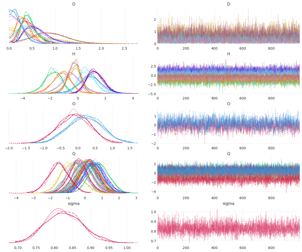
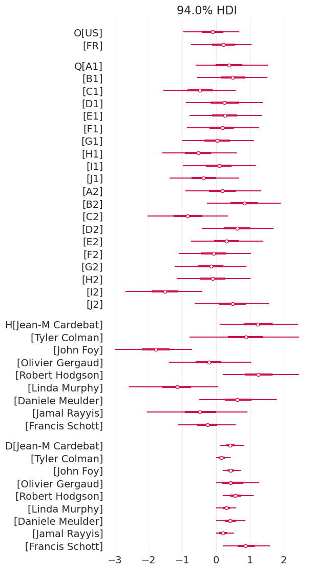
后验摘要#
az.plot_forest(judges_inference, var_names=["O", "Q", "H", "D"], combined=True);
葡萄酒产地重要吗?#
_, ax = plt.subplots(figsize=(4, 2))
az.plot_forest(judges_inference, combined=True, var_names=["O"], ax=ax);
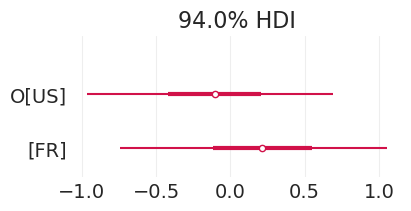
并非真的重要,至少在比较葡萄酒产地的后验变量 \(O\) 时是这样
计算对比分布#
始终进行对比#
# Posterior contrast
plt.subplots(figsize=(6, 3))
quality_US = judges_inference.posterior.sel(wine_origin="US")
quality_FR = judges_inference.posterior.sel(wine_origin="FR")
contrast = quality_US - quality_FR

wine_origin_model_param = "O"

az.plot_dist(contrast[wine_origin_model_param], label="Quality Contrast\n(US - FR)")
plt.axvline(0, color="k", linestyle="--", label="No Difference")
plt.xlabel("origin contrast")
plt.ylabel("density")
plt.legend();
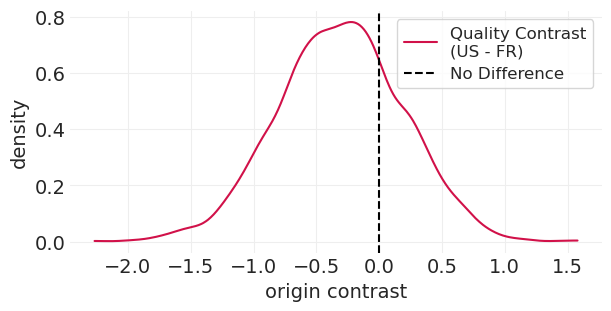
后验对比支持相同的结果。新泽西州和法国葡萄酒的质量几乎没有差异(如果有的话)。
Gelman 的智慧之言#
当您遇到计算问题时,通常是您的模型存在问题。
注意
模型的科学假设
先验
变量预处理
采样器设置
警惕发散
这些是违反哈密顿条件 HMC 模拟;不可靠的提议
发散通常是模型设计不正确或可以参数化以提高采样效率(例如,非中心先验)的症状
向 Spiegelhalter 致敬!🐞🐛🪲#
BUGS 包启动了桌面 MCMC 革命
许可声明#
此示例 галерея 中的所有笔记本均根据 MIT 许可证 提供,该许可证允许修改和再分发以用于任何用途,前提是保留版权和许可声明。
引用 PyMC 示例#
要引用此笔记本,请使用 Zenodo 为 pymc-examples 存储库提供的 DOI。
重要提示
许多笔记本改编自其他来源:博客、书籍... 在这种情况下,您也应引用原始来源。
还请记住引用您的代码使用的相关库。
这是一个 bibtex 中的引用模板
@incollection{citekey,
  author    = "<notebook authors, see above>",
  title     = "<notebook title>",
  editor    = "PyMC Team",
  booktitle = "PyMC examples",
  doi       = "10.5281/zenodo.5654871"
}
一旦呈现,它可能看起来像
社交网络#
从人或群体 \(A\) 到 \(B\) 的关系 \(R_{AB}\) 可能会导致涉及 \(Y_{AB}\) 的某些结果
例如,\(A\) 可能是 \(B\) 的崇拜者
类似地,但不一定是对称地,\(R_{BA}\) 可能会导致涉及 \(Y_{AB}\) 的某些结果
例如,\(B\) 可能不是 \(A\) 的崇拜者
人或群体的特征 \(X_*\) 也会影响关系和结果
例如,\(A\) 和/或 \(B\) 的财富状况
互动 \(Y_*\) 不会发生在其他某人或群体 \(C\) 之间
所有这些非结果变量都可能是未观察到的
因为某些社交互动结构。鉴于我们只能衡量其中一些结果,我们必须推断网络结构