


建模事件#
此笔记本是 PyMC 端口的一部分,该端口移植自 Richard McElreath 的 Statistical Rethinking 2023 系列讲座。
视频 - 第 09 讲 - 建模事件# 第 09 讲 - 建模事件
# Ignore warnings
import warnings

import arviz as az
import numpy as np
import pandas as pd
import pymc as pm
import statsmodels.formula.api as smf
import utils as utils
import xarray as xr

from matplotlib import pyplot as plt
from matplotlib import style
from scipy import stats as stats

warnings.filterwarnings("ignore")

# Set matplotlib style
STYLE = "statistical-rethinking-2023.mplstyle"
style.use(STYLE)
加州大学伯克利分校录取#
数据集#
4562 名研究生申请者
按以下因素分层:
院系
性别
目标是识别招生官的性别歧视
ADMISSIONS = utils.load_data("UCBadmit")
ADMISSIONS
| 院系 | 申请者性别 | 录取 | 拒绝 | 申请数 | |
|---|---|---|---|---|---|
| 1 | A | 男性 | 512 | 313 | 825 |
| 2 | A | 女性 | 89 | 19 | 108 |
| 3 | B | 男性 | 353 | 207 | 560 |
| 4 | B | 女性 | 17 | 8 | 25 |
| 5 | C | 男性 | 120 | 205 | 325 |
| 6 | C | 女性 | 202 | 391 | 593 |
| 7 | D | 男性 | 138 | 279 | 417 |
| 8 | D | 女性 | 131 | 244 | 375 |
| 9 | E | 男性 | 53 | 138 | 191 |
| 10 | E | 女性 | 94 | 299 | 393 |
| 11 | F | 男性 | 22 | 351 | 373 |
| 12 | F | 女性 | 24 | 317 | 341 |
建模事件#
事件:离散、无序的结果
观测是计数/聚合
未知数是事件发生的概率 \(p\),或这些概率的几率 \(\frac{p}{1-p}\)
我们分层的全部事物都会相互作用——在现实生活中通常不是独立的
通常处理 \(p = \log \left (\frac{p}{1-p} \right)\) 的对数几率
招生:画猫头鹰 🦉#
估计量
科学模型
统计模型
分析
1. 估计量#
哪条路径定义了“歧视”#
直接歧视(因果效应)#
utils.draw_causal_graph(
    edge_list=[("G", "D"), ("G", "A"), ("D", "A")],
    node_props={
        "G": {"label": "Gender, G", "color": "red"},
        "D": {"label": "Department, D"},
        "A": {"label": "Admission rate, A", "color": "red"},
    },
    edge_props={("G", "A"): {"color": "red"}},
    graph_direction="LR",
)

又称“制度性歧视”
裁判对特定群体有偏见
通常是我们有兴趣识别是否存在的类型
需要强因果假设
在此,院系 D 是一个中介——这是社会科学中常见的结构,其中分类地位(例如,性别)影响某些中介背景(例如,职业),两者都会影响目标结果(工资)。示例
工资歧视
招聘
科学奖项
间接歧视#
utils.draw_causal_graph(
    edge_list=[("G", "D"), ("G", "A"), ("D", "A")],
    node_props={
        "G": {"label": "Gender, G", "color": "red"},
        "D": {"label": "Department, D"},
        "A": {"label": "Admission rate, A", "color": "red"},
    },
    edge_props={("G", "D"): {"color": "red"}, ("D", "A"): {"color": "red"}},
    graph_direction="LR",
)

又称“结构性歧视”
例如,性别影响一个人的兴趣,从而影响他们将申请的院系
影响总体录取率
需要强因果假设
总歧视#
utils.draw_causal_graph(
    edge_list=[("G", "D"), ("G", "A"), ("D", "A")],
    node_props={
        "G": {"label": "Gender, G", "color": "red"},
        "D": {"label": "Department, D"},
        "A": {"label": "Admission rate, A", "color": "red"},
    },
    edge_props={
        ("G", "D"): {"color": "red"},
        ("G", "A"): {"color": "red"},
        ("D", "A"): {"color": "red"},
    },
    graph_direction="LR",
)

又称“经验性歧视”
通过直接和间接途径
需要温和的假设
估计量 & 估计器#
每个 不同的估计量都需要不同的估计器
通常我们 可以估计 的东西往往不是我们 想要估计 的东西
例如,总歧视可能更容易估计,但可操作性较差
未观测到的混淆因素#
utils.draw_causal_graph(
    edge_list=[("G", "D"), ("G", "A"), ("D", "A"), ("U", "D"), ("U", "A")],
    node_props={"U": {"style": "dashed"}, "unobserved": {"style": "dashed"}},
    graph_direction="LR",
)

总是可能在中介和某些未观测到的混淆因素之间也存在混淆。我们现在将忽略这些。
2. 科学模型:#
模拟过程#
下面是审查/录取过程的生成模型
np.random.seed(123)
n_samples = 1000

GENDER = stats.bernoulli.rvs(p=0.5, size=n_samples)

# Groundtruth parameters
# Gender 1 tends to apply to department 1
P_DEPARTMENT = np.where(GENDER == 0, 0.3, 0.8)

# Acceptance rates matrices -- Department x Gender
UNBIASED_ACCEPTANCE_RATES = np.array([[0.1, 0.1], [0.3, 0.3]])  # No *direct* gender bias

# Biased acceptance:
# - dept 0 accepts gender 0 at 50% of unbiased rate
# - dept 1 accepts gender 0 at 67% of unbiased rate
BIASED_ACCEPTANCE_RATES = np.array([[0.05, 0.1], [0.2, 0.3]])  # *direct* gender bias present

DEPARTMENT = stats.bernoulli.rvs(p=P_DEPARTMENT, size=n_samples).astype(int)


def simulate_admissions_data(bias_type):
    """Simulate admissions data using the global params above"""
    acceptance_rate = (
        BIASED_ACCEPTANCE_RATES if bias_type == "biased" else UNBIASED_ACCEPTANCE_RATES
    )
    acceptance = stats.bernoulli.rvs(p=acceptance_rate[DEPARTMENT, GENDER])

    return (
        pd.DataFrame(
            np.vstack([GENDER, DEPARTMENT, acceptance]).T,
            columns=["gender", "department", "accepted"],
        ),
        acceptance_rate,
    )


for bias_type in ["unbiased", "biased"]:

    fake_admissions, acceptance_rate = simulate_admissions_data(bias_type)

    gender_acceptance_counts = fake_admissions.groupby(["gender", "accepted"]).count()["department"]
    gender_acceptance_counts.name = None

    gender_department_counts = fake_admissions.groupby(["gender", "department"]).count()["accepted"]
    gender_department_counts.name = None

    observed_acceptance_rates = fake_admissions.groupby("gender").mean()["accepted"]
    observed_acceptance_rates.name = None

    print()
    print("-" * 30)
    print(bias_type.upper())
    print("-" * 30)
    print(f"Department Acceptance rate:\n{acceptance_rate}")
    print(f"\nGender-Department Frequency:\n{gender_department_counts}")
    print(f"\nGender-Acceptance Frequency:\n{gender_acceptance_counts}")
    print(f"\nOverall Acceptance Rates:\n{observed_acceptance_rates}")
------------------------------
UNBIASED
------------------------------
Department Acceptance rate:
[[0.1 0.1]
 [0.3 0.3]]

Gender-Department Frequency:
gender  department
0       0             335
        1             173
1       0             106
        1             386
dtype: int64

Gender-Acceptance Frequency:
gender  accepted
0       0           437
        1            71
1       0           359
        1           133
dtype: int64

Overall Acceptance Rates:
gender
0    0.139764
1    0.270325
dtype: float64

------------------------------
BIASED
------------------------------
Department Acceptance rate:
[[0.05 0.1 ]
 [0.2  0.3 ]]

Gender-Department Frequency:
gender  department
0       0             335
        1             173
1       0             106
        1             386
dtype: int64

Gender-Acceptance Frequency:
gender  accepted
0       0           465
        1            43
1       0           370
        1           122
dtype: int64

Overall Acceptance Rates:
gender
0    0.084646
1    0.247967
dtype: float64
模拟数据属性#
两种情景#
性别 0 倾向于申请院系 0
性别 1 倾向于申请院系 1
无偏情景:#
由于院系 0 的录取率较低,并且性别 0 倾向于申请院系 0,因此性别 0 的总体拒绝率低于性别 1
由于院系 1 的录取率较高,并且性别 1 倾向于申请院系 1,因此性别 1 的总体录取率高于性别 0
即使在没有(直接)性别歧视的情况下,仍然存在基于性别倾向于申请不同院系的间接歧视,以及每个院系录取学生的不均等可能性。
有偏情景#
总体录取率较低(由于性别 0 在两个院系的录取率均有所降低)
在存在实际院系偏见的情景中,由于间接效应,我们看到与无偏情况类似的总体歧视模式。
3. 统计模型#
建模事件#
我们观察到 事件的计数
我们估计 概率——或者,更确切地说,是事件发生的对数几率
线性模型#
期望值是参数的线性(加性)组合
b.c. 正态分布是无界的,因此线性模型的期望值也是无界的。
事件模型#
离散事件要么发生,取值 1,要么不发生,取值 0。这 对 事件的期望值 设置了界限。即界限在区间 \((0, 1)\) 内
广义线性模型 & 链接函数#
期望值是 参数的加性组合的某个函数 \(f(\mathbb{E}[\theta])\) 。
通常,此函数 \(f()\),称为 链接函数,将具有与 似然分布相关的 特定形式。
链接函数将具有 逆链接函数 \( f^{-1}(X_i, \theta)\),使得
重申一下,链接函数与分布相匹配
在线性回归情况下,似然模型是高斯的,并且相关的链接函数(和逆链接函数)只是恒等函数,\(I()\)。(左图如下)
_, axs = plt.subplots(1, 2, figsize=(8, 4))
xs = np.linspace(-3, 3, 100)
plt.sca(axs[0])
alpha = 0
beta = 0.75

plt.plot(xs, alpha + beta * xs)
plt.axhline([0], linestyle="--", color="gray")
plt.axhline([1], linestyle="--", color="gray")
plt.xlim([-3, 3])
plt.ylim([-0.5, 1.5])
plt.xlabel("x")
plt.ylabel("$I(\\alpha + \\beta X$)")
plt.title("Linear Model\n(continous outcomes)")

plt.sca(axs[1])
plt.plot(xs, utils.invlogit(alpha + beta * xs))
plt.axhline([0], linestyle="--", color="gray")
plt.axhline([1], linestyle="--", color="gray")
plt.xlim([-3, 3])
plt.ylim([-0.5, 1.5])
plt.xlabel("x")
plt.ylabel("$\\frac{1}{e^{-(\\alpha + \\beta X)}}$")
plt.title("Logistic Model\n(binary outcomes)");
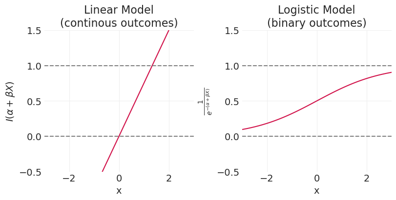
Logit 链接函数和 Logistic 逆函数#
二元结果#
逻辑回归 用于建模事件发生的概率
似然函数是伯努利分布
相关的链接函数是 对数几率,或 logit:\(f(p) = \frac{p}{1-p}\)
逆链接函数是 逆 logit 又名 logistic 函数(上图右侧):\(f^{-1}(X_i, \theta) = \frac{1}{1 + e^{-(\alpha + \beta_X X_i + ...)}}\)
定义 \(\alpha + \beta_X X + ... = q\) (暂时忽略数据索引 \(i\)),逆 logit 的推导如下
\[\begin{split} \begin{align} \log \left(\frac{p}{1-p}\right) &= \alpha + \beta_X X + ... = q \\ \frac{p}{1-p} &= e^{q} \\ p &= (1-p) e^{q} \\ p + p e^{q} &= e^{q} \\ p(1 + e^{q}) &= e^{q} \\ p &= \frac{ e^{q}}{(1 + e^{q})} \\ p &= \frac{ e^{q}}{(1 + e^{q})} \frac{e^{-q}}{e^{-q}}\\ p &= \frac{1}{(1 + e^{-q})} \\ \end{align} \end{split}\]
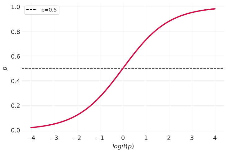
logit 是一种苛刻的变换#
最初解释对数几率可能很困难,但随着时间的推移会变得更容易
对数几率尺度
\(\text{logit}(p)=0, p=0.5\)
\(\text{logit}(p)=-\infty, p=0\)
经验法则:\(\text{logit}(p)<-4\) 意味着事件不太可能发生(几乎从不)
\(\text{logit}(p)=\infty, p=1\)
经验法则:\(\text{logit}(p)>4\) 意味着事件非常可能发生(几乎总是)
log_odds = np.linspace(-4, 4, 100)
utils.plot_line(log_odds, utils.invlogit(log_odds), label=None)
plt.axhline(0.5, linestyle="--", color="k", label="p=0.5")
plt.xlabel("$logit(p)$")
plt.ylabel("$p$")
plt.legend();
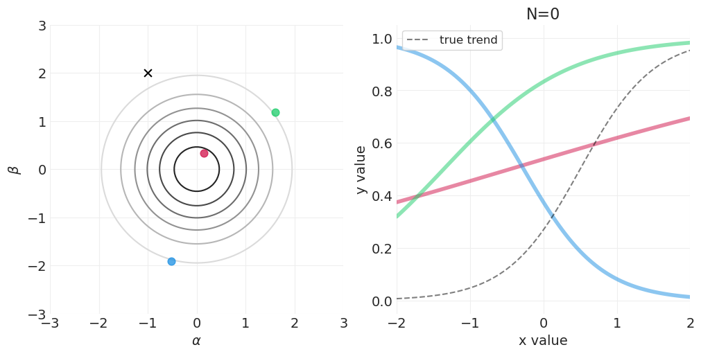
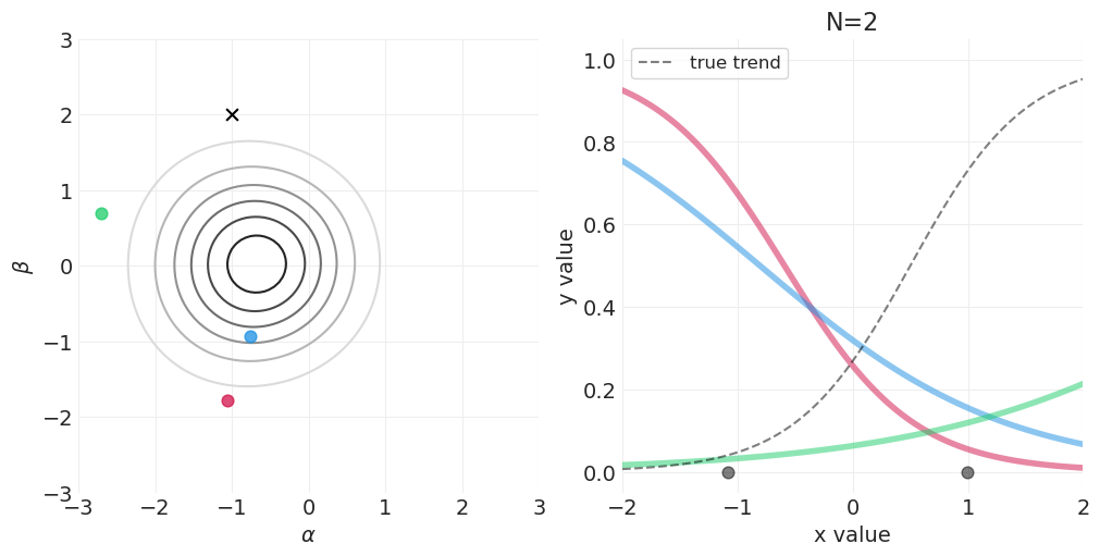
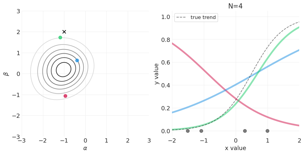
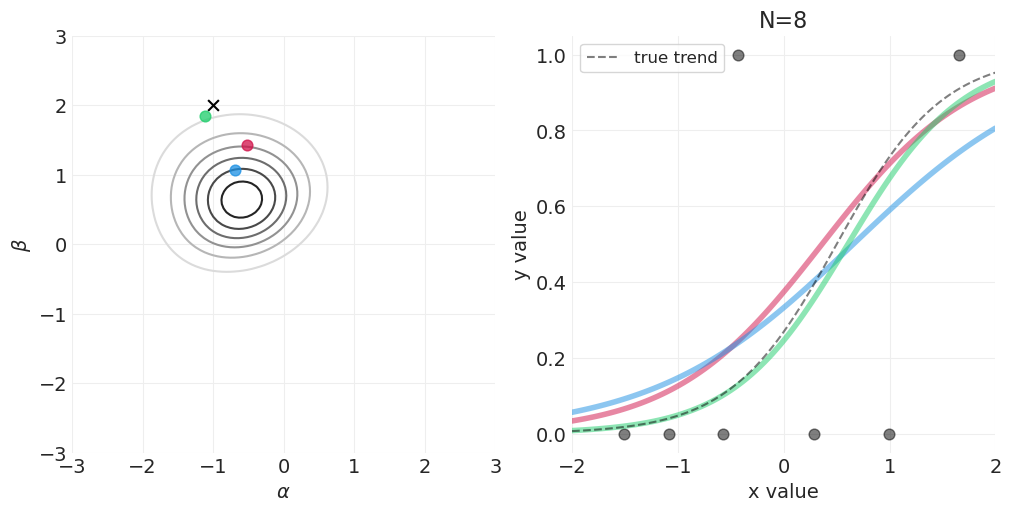
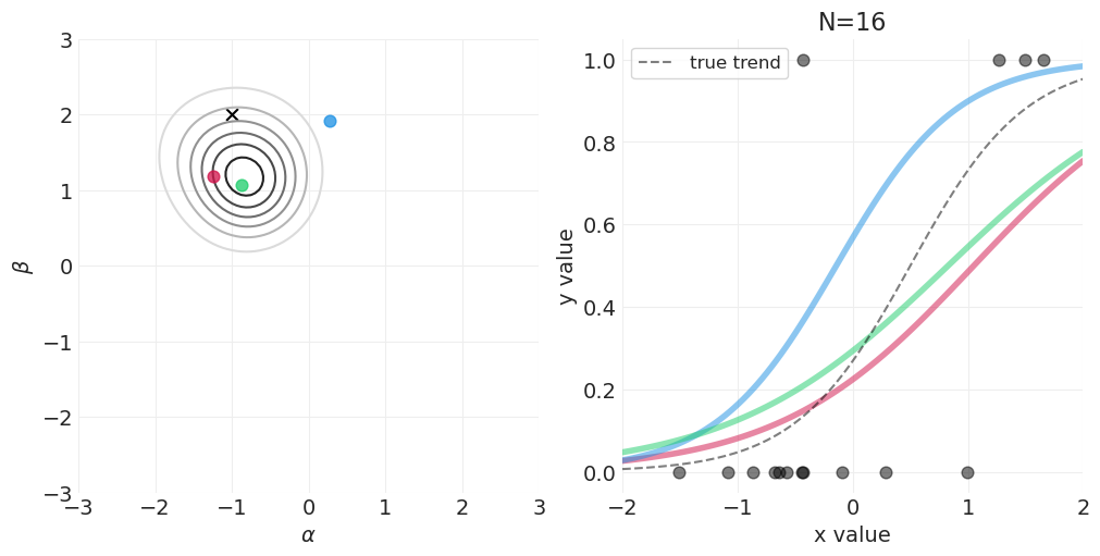
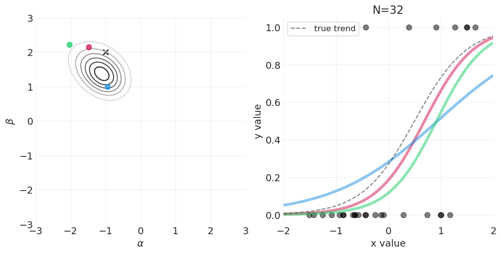
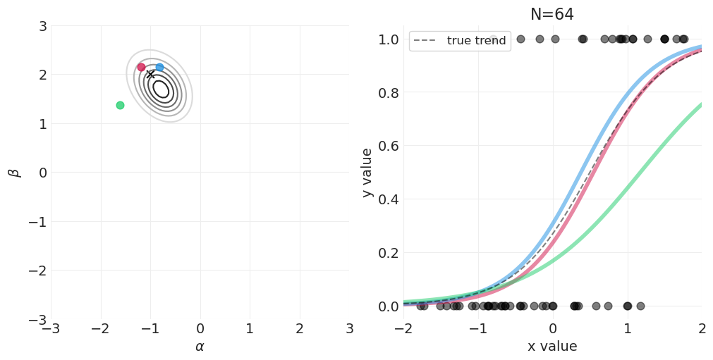
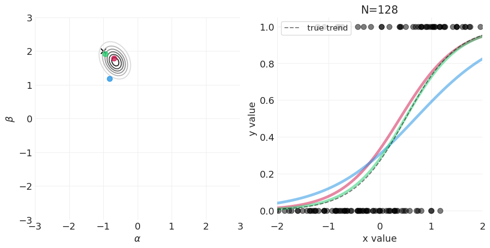
逻辑回归的贝叶斯更新#
对于以下模拟,我们将使用自定义实用函数 utils.simulate_2_parameter_bayesian_learning 来模拟一般的贝叶斯后验更新模拟。以下是该函数的 API(有关更多详细信息,请参见 utils.py)
help(utils.simulate_2_parameter_bayesian_learning_grid_approximation)
Help on function simulate_2_parameter_bayesian_learning_grid_approximation in module utils:

simulate_2_parameter_bayesian_learning_grid_approximation(x_obs, y_obs, param_a_grid, param_b_grid, true_param_a, true_param_b, model_func, posterior_func, n_posterior_samples=3, param_labels=None, data_range_x=None, data_range_y=None)
    General function for simulating Bayesian learning in a 2-parameter model
    using grid approximation.

    Parameters
    ----------
    x_obs : np.ndarray
        The observed x values
    y_obs : np.ndarray
        The observed y values
    param_a_grid: np.ndarray
        The range of values the first model parameter in the model can take.
        Note: should have same length as param_b_grid.
    param_b_grid: np.ndarray
        The range of values the second model parameter in the model can take.
        Note: should have same length as param_a_grid.
    true_param_a: float
        The true value of the first model parameter, used for visualizing ground
        truth
    true_param_b: float
        The true value of the second model parameter, used for visualizing ground
        truth
    model_func: Callable
        A function `f` of the form `f(x, param_a, param_b)`. Evaluates the model
        given at data points x, given the current state of parameters, `param_a`
        and `param_b`. Returns a scalar output for the `y` associated with input
        `x`.
    posterior_func: Callable
        A function `f` of the form `f(x_obs, y_obs, param_grid_a, param_grid_b)
        that returns the posterior probability given the observed data and the
        range of parameters defined by `param_grid_a` and `param_grid_b`.
    n_posterior_samples: int
        The number of model functions sampled from the 2D posterior
    param_labels: Optional[list[str, str]]
        For visualization, the names of `param_a` and `param_b`, respectively
    data_range_x: Optional len-2 float sequence
        For visualization, the upper and lower bounds of the domain used for model
        evaluation
    data_range_y: Optional len-2 float sequence
        For visualization, the upper and lower bounds of the range used for model
        evaluation.
# Model function required for simulation


def logistic_model(x, alpha, beta):
    return utils.invlogit(alpha + beta * x)


# Posterior function required for simulation
def logistic_regression_posterior(x_obs, y_obs, alpha_grid, beta_grid, likelihood_prior_std=0.01):

    # Convert params to 1-d arrays
    if np.ndim(alpha_grid) > 1:
        alpha_grid = alpha_grid.ravel()

    if np.ndim(beta_grid):
        beta_grid = beta_grid.ravel()

    log_prior_intercept = stats.norm(0, 1).logpdf(alpha_grid)
    log_prior_slope = stats.norm(0, 1).logpdf(beta_grid)

    log_likelihood = np.array(
        [
            stats.bernoulli(p=utils.invlogit(a + b * x_obs)).logpmf(y_obs)
            for a, b in zip(alpha_grid, beta_grid)
        ]
    ).sum(axis=1)

    # Posterior is equal to the product of likelihood and priors (here a sum in log scale)
    log_posterior = log_likelihood + log_prior_intercept + log_prior_slope

    # Convert back to natural scale
    return np.exp(log_posterior - log_posterior.max())


# Generate data for demo
np.random.seed(123)
RESOLUTION = 100
N_DATA_POINTS = 128

# Ground truth parameters
ALPHA = -1
BETA = 2

x = stats.norm(0, 1).rvs(size=N_DATA_POINTS)
p_y = utils.invlogit(ALPHA + BETA * x)
y = stats.bernoulli.rvs(p=p_y)

alpha_grid = np.linspace(-3, 3, RESOLUTION)
beta_grid = np.linspace(-3, 3, RESOLUTION)

# Vary the sample size to show how the posterior adapts to more and more data
for n_samples in [0, 2, 4, 8, 16, 32, 64, 128]:
    # Run the simulation
    utils.simulate_2_parameter_bayesian_learning_grid_approximation(
        x_obs=x[:n_samples],
        y_obs=y[:n_samples],
        param_a_grid=alpha_grid,
        param_b_grid=beta_grid,
        true_param_a=ALPHA,
        true_param_b=BETA,
        model_func=logistic_model,
        posterior_func=logistic_regression_posterior,
        param_labels=["$\\alpha$", "$\\beta$"],
        data_range_x=(-2, 2),
        data_range_y=(-0.05, 1.05),
    )
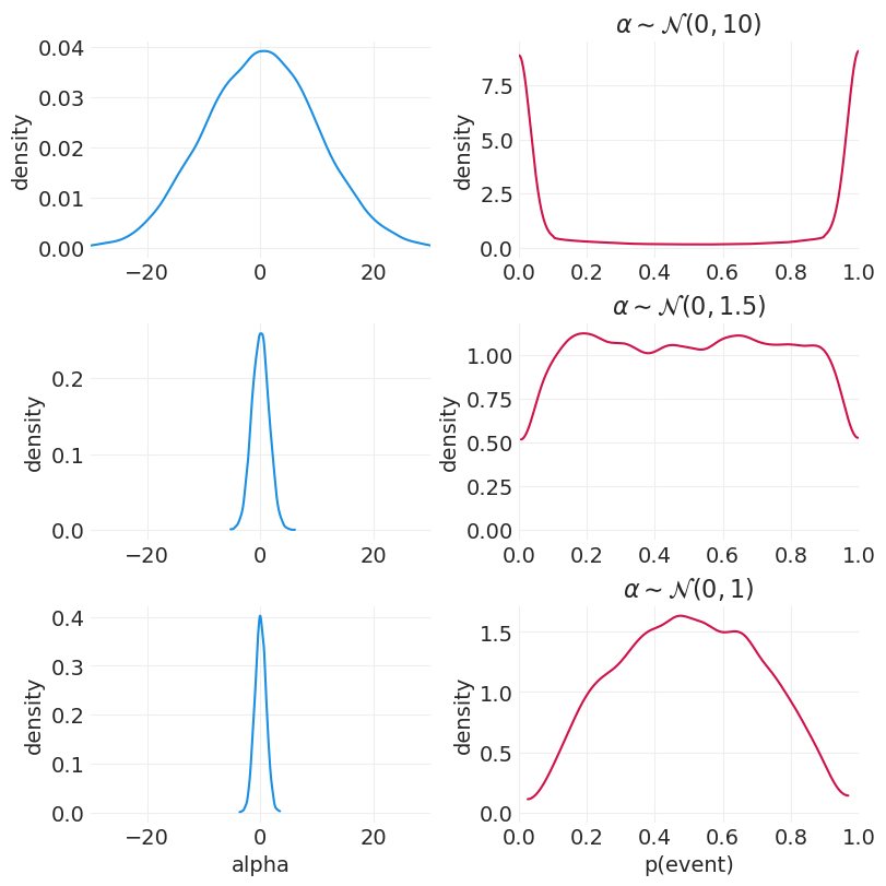
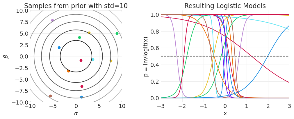
逻辑回归的先验#
logit 链接函数是一种苛刻的变换
Logit 压缩参数分布
\(x > +4 \rightarrow \) 事件基本上总是发生
\(x < -4 \rightarrow\) 事件基本上从不发生
n_samples = 10000
fig, axs = plt.subplots(3, 2, figsize=(8, 8))
for ii, std in enumerate([10, 1.5, 1]):

    # Alpha prior distribution
    alphas = stats.norm(0, std).rvs(n_samples)
    plt.sca(axs[ii][0])
    az.plot_dist(alphas, color="C1")
    plt.xlim([-30, 30])
    plt.ylabel("density")
    if ii == 2:
        plt.xlabel("alpha")

    # Resulting event probability distribution
    ps = utils.invlogit(alphas)
    plt.sca(axs[ii][1])
    az.plot_dist(ps, color="C0")
    plt.xlim([0, 1])
    plt.ylabel("density")
    plt.title(f"$\\alpha \sim \mathcal{{N}}(0, {std})$")
    if ii == 2:
        plt.xlabel("p(event)")
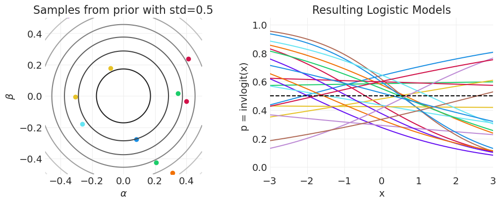
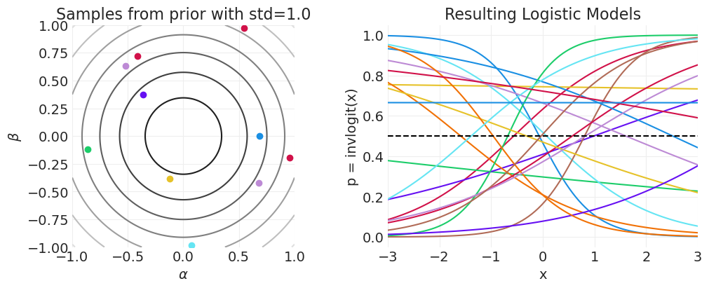
先验预测模拟#
# Demonstrating the effect of alpha / beta on p(x)
from functools import partial


def gaussian_2d_pdf(xs, ys, mean=(0, 0), covariance=np.eye(2)):
    return np.array(stats.multivariate_normal(mean, covariance).pdf(np.vstack([xs, ys]).T))


pdf = partial(gaussian_2d_pdf)

xs = ys = np.linspace(-3, 3, 100)
# utils.plot_2d_function(xs, ys, pdf, cmap='gray_r')


def plot_logistic_prior_predictive(n_samples=20, prior_std=0.5):

    _, axs = plt.subplots(1, 2, figsize=(10, 4))
    plt.sca(axs[0])
    min_x, max_x = -prior_std, prior_std
    xs = np.linspace(min_x, max_x, 100)
    ys = xs

    pdf = partial(gaussian_2d_pdf, covariance=np.array([[prior_std**2, 0], [0, prior_std**2]]))
    utils.plot_2d_function(xs, ys, pdf, cmap="gray_r")

    plt.axis("square")
    plt.xlim([min_x, max_x])
    plt.ylim([min_x, max_x])

    # Sample some parameters from prior
    βs = stats.norm.rvs(0, prior_std, size=n_samples)
    αs = stats.norm.rvs(0, prior_std, size=n_samples)

    for b, a in zip(βs, αs):
        plt.scatter(a, b)

    plt.xlabel("$\\alpha$")
    plt.ylabel("$\\beta$")
    plt.title(f"Samples from prior with std={prior_std}")

    # Resulting sigmoid functions
    plt.sca(axs[1])
    min_x, max_x = -3, 3
    xs = np.linspace(min_x, max_x, 100)
    for a, b in zip(αs, βs):
        logit_p = a + xs * b
        p = utils.invlogit(logit_p)
        plt.plot(xs, p)

    plt.xlabel("x")
    plt.ylabel("p = invlogit(x)")
    plt.xlim([-3, 3])
    plt.ylim([-0.05, 1.05])
    plt.axhline(0.5, linestyle="--", color="k")
    plt.title(f"Resulting Logistic Models")
plot_logistic_prior_predictive(prior_std=0.5)
plot_logistic_prior_predictive(prior_std=1.0)
plot_logistic_prior_predictive(prior_std=10)
招生统计模型#
同样,估计器将取决于估计量
总因果效应#
utils.draw_causal_graph(
    edge_list=[("G", "D"), ("G", "A"), ("D", "A")],
    node_props={
        "G": {"color": "red"},
        "A": {"color": "red"},
    },
    edge_props={
        ("G", "A"): {"color": "red"},
        ("D", "A"): {"color": "red"},
        ("G", "D"): {"color": "red"},
    },
    graph_direction="LR",
)

仅按性别分层。不要按院系分层,因为它是我们不想阻止的管道(中介)
直接因果效应#
utils.draw_causal_graph(
    edge_list=[("G", "D"), ("G", "A"), ("D", "A")],
    node_props={
        "G": {"color": "red"},
        "A": {"color": "red"},
    },
    edge_props={("G", "A"): {"color": "red"}},
    graph_direction="LR",
)

按性别和院系分层 以阻止管道
拟合总因果效应模型#
def fit_total_effect_model_admissions(data):
"""Fit total effect model, stratifying by gender.
Note
----
We use the Binomial regression, so simulated observation-level
data from above must be pre-aggregated. (see the function
`aggregate_admissions_data` below). We could have
used a Bernoulli likelihood (Logistic regression) for the simulated
data, but given that we only have aggregates for the real
UC Berkeley data we choose this more general formulation.
"""
# Set up observations / coords
n_admitted = data["admit"].values
n_applications = data["applications"].values
gender_coded, gender = pd.factorize(data["applicant.gender"].values)
with pm.Model(coords={"gender": gender}) as total_effect_model:
# Mutable data for running any gender-based counterfactuals
gender_coded = pm.Data("gender", gender_coded, dims="obs_ids")
alpha = pm.Normal("alpha", 0, 1, dims="gender")
# Record the inverse linked probabilities for reporting
pm.Deterministic("p_accept", pm.math.invlogit(alpha), dims="gender")
p = pm.math.invlogit(alpha[gender_coded])
likelihood = pm.Binomial(
"accepted", n=n_applications, p=p, observed=n_admitted, dims="obs_ids"
)
total_effect_inference = pm.sample()
return total_effect_model, total_effect_inference
def aggregate_admissions_data(raw_admissions_data):
"""Aggregate simulated data from `simulate_admissions_data`, which
is in long format to short format, by so that it can be modeled
using Binomial likelihood. We also recode column names to have the
same fields as the UC Berkeley dataset so that we can use the
same model-fitting functions.
"""
# Aggregate applications, admissions, and rejections. Rename
# columns to have the same fields as UC Berkeley dataset
applications = raw_admissions_data.groupby(["gender", "department"]).count().reset_index()
applications.rename(columns={"accepted": "applications"}, inplace=True)
admits = raw_admissions_data.groupby(["gender", "department"]).sum().reset_index()
admits.rename(columns={"accepted": "admit"}, inplace=True)
data = applications.merge(admits)
data.loc[:, "reject"] = data.applications - data.admit
# Code gender & department. For easier comparison to lecture,
# we use 1-indexed gender/department indicators like McElreath
data.loc[:, "applicant.gender"] = data.gender.apply(lambda x: 2 if x else 1)
data.loc[:, "dept"] = data.department.apply(lambda x: 2 if x else 1)
return data[["applicant.gender", "dept", "applications", "admit", "reject"]]
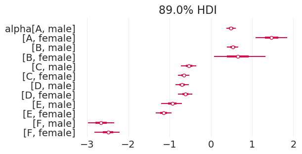
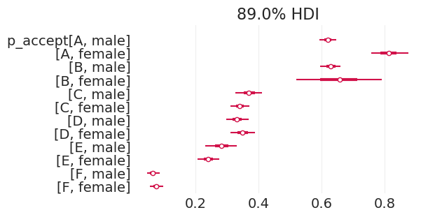
def plot_admissions_model_posterior(inference, figsize=(6, 2)):
_, ax = plt.subplots(figsize=figsize)
# Plot alphas
az.plot_forest(inference, var_names=["alpha"], combined=True, hdi_prob=0.89, ax=ax)
# Plot inver-linked acceptance probabilities
_, ax = plt.subplots(figsize=figsize)
az.plot_forest(inference, var_names=["p_accept"], combined=True, hdi_prob=0.89, ax=ax)
return az.summary(inference)
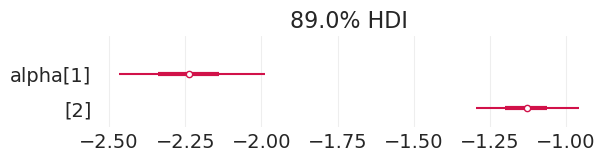
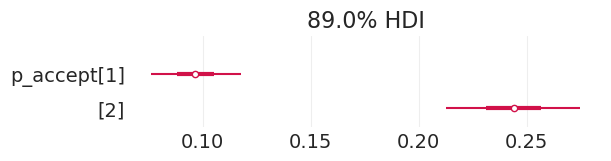
在有偏模拟招生数据上拟合总效应模型#
SIMULATED_BIASED_ADMISSIONS, _ = simulate_admissions_data("biased")
SIMULATED_BIASED_ADMISSIONS = aggregate_admissions_data(SIMULATED_BIASED_ADMISSIONS)
SIMULATED_BIASED_ADMISSIONS
| 申请者性别 | 院系 | 申请数 | 录取 | 拒绝 | |
|---|---|---|---|---|---|
| 0 | 1 | 1 | 335 | 13 | 322 |
| 1 | 1 | 2 | 173 | 34 | 139 |
| 2 | 2 | 1 | 106 | 11 | 95 |
| 3 | 2 | 2 | 386 | 108 | 278 |
total_effect_model_simulated_biased, total_effect_inference_simulated_biased = (
    fit_total_effect_model_admissions(SIMULATED_BIASED_ADMISSIONS)
)
Initializing NUTS using jitter+adapt_diag...
Multiprocess sampling (4 chains in 4 jobs)
NUTS: [alpha]
Sampling 4 chains for 1_000 tune and 1_000 draw iterations (4_000 + 4_000 draws total) took 1 seconds.
plot_admissions_model_posterior(total_effect_inference_simulated_biased, (6, 1.5))
| 均值 | 标准差 | HDI_3% | HDI_97% | MCSE_均值 | MCSE_标准差 | ESS_批量 | ESS_尾部 | R_hat | |
|---|---|---|---|---|---|---|---|---|---|
| alpha[1] | -2.240 | 0.151 | -2.531 | -1.958 | 0.002 | 0.002 | 3876.0 | 2626.0 | 1.0 |
| alpha[2] | -1.133 | 0.106 | -1.335 | -0.939 | 0.002 | 0.001 | 4108.0 | 3100.0 | 1.0 |
| p_accept[1] | 0.097 | 0.013 | 0.071 | 0.121 | 0.000 | 0.000 | 3876.0 | 2626.0 | 1.0 |
| p_accept[2] | 0.244 | 0.019 | 0.208 | 0.281 | 0.000 | 0.000 | 4108.0 | 3100.0 | 1.0 |
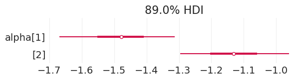
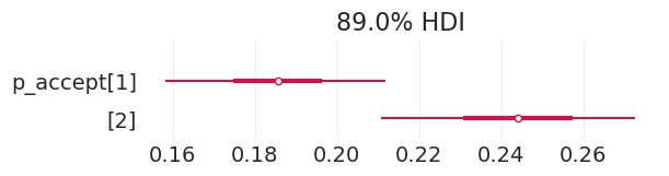
在无偏模拟招生数据上拟合总效应模型#
SIMULATED_UNBIASED_ADMISSIONS, _ = simulate_admissions_data("unbiased")
SIMULATED_UNBIASED_ADMISSIONS = aggregate_admissions_data(SIMULATED_UNBIASED_ADMISSIONS)
SIMULATED_UNBIASED_ADMISSIONS
| 申请者性别 | 院系 | 申请数 | 录取 | 拒绝 | |
|---|---|---|---|---|---|
| 0 | 1 | 1 | 335 | 33 | 302 |
| 1 | 1 | 2 | 173 | 60 | 113 |
| 2 | 2 | 1 | 106 | 8 | 98 |
| 3 | 2 | 2 | 386 | 111 | 275 |
total_effect_model_simulated_unbiased, total_effect_inference_simulated_unbiased = (
    fit_total_effect_model_admissions(SIMULATED_UNBIASED_ADMISSIONS)
)
Initializing NUTS using jitter+adapt_diag...
Multiprocess sampling (4 chains in 4 jobs)
NUTS: [alpha]
Sampling 4 chains for 1_000 tune and 1_000 draw iterations (4_000 + 4_000 draws total) took 1 seconds.
plot_admissions_model_posterior(total_effect_inference_simulated_unbiased, (6, 1.5))
| 均值 | 标准差 | HDI_3% | HDI_97% | MCSE_均值 | MCSE_标准差 | ESS_批量 | ESS_尾部 | R_hat | |
|---|---|---|---|---|---|---|---|---|---|
| alpha[1] | -1.481 | 0.112 | -1.694 | -1.264 | 0.002 | 0.001 | 3700.0 | 2457.0 | 1.0 |
| alpha[2] | -1.132 | 0.107 | -1.327 | -0.937 | 0.002 | 0.001 | 4389.0 | 2864.0 | 1.0 |
| p_accept[1] | 0.186 | 0.017 | 0.150 | 0.215 | 0.000 | 0.000 | 3700.0 | 2457.0 | 1.0 |
| p_accept[2] | 0.244 | 0.020 | 0.210 | 0.281 | 0.000 | 0.000 | 4389.0 | 2864.0 | 1.0 |
拟合直接因果效应模型#
def fit_direct_effect_model_admissions(data):
    """Fit total effect model, stratifying by gender.

    Note
    ----
    We use the Binomial likelihood, so simulated observation-level data from
    above must be pre-aggregated. (see the function `aggregate_admissions_data`
    below). We could have used a Bernoulli likelihood for the simulated data,
    but given that we only have aggregates for the real UC Berkeley data we
    choose this more general formulation.
    """

    # Set up observations / coords
    n_admitted = data["admit"].values
    n_applications = data["applications"].values

    department_coded, department = pd.factorize(data["dept"].values)
    gender_coded, gender = pd.factorize(data["applicant.gender"].values)

    with pm.Model(coords={"gender": gender, "department": department}) as direct_effect_model:

        # Mutable data for running any gender-based or department-based counterfactuals
        gender_coded = pm.Data("gender", gender_coded, dims="obs_ids")
        department_coded = pm.Data("department", department_coded, dims="obs_ids")
        n_applications = pm.Data("n_applications", n_applications, dims="obs_ids")

        alpha = pm.Normal("alpha", 0, 1, dims=["department", "gender"])

        # Record inverse linked probabilities for reporting
        pm.Deterministic("p_accept", pm.math.invlogit(alpha), dims=["department", "gender"])

        p = pm.math.invlogit(alpha[department_coded, gender_coded])

        likelihood = pm.Binomial(
            "accepted", n=n_applications, p=p, observed=n_admitted, dims="obs_ids"
        )
        direct_effect_inference = pm.sample()

    return direct_effect_model, direct_effect_inference
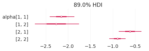
将直接效应模型拟合到有偏模拟招生数据#
direct_effect_model_simulated_biased, direct_effect_inference_simulated_biased = (
    fit_direct_effect_model_admissions(SIMULATED_BIASED_ADMISSIONS)
)
Initializing NUTS using jitter+adapt_diag...
Multiprocess sampling (4 chains in 4 jobs)
NUTS: [alpha]
Sampling 4 chains for 1_000 tune and 1_000 draw iterations (4_000 + 4_000 draws total) took 1 seconds.
plot_admissions_model_posterior(direct_effect_inference_simulated_biased)
| 均值 | 标准差 | HDI_3% | HDI_97% | MCSE_均值 | MCSE_标准差 | ESS_批量 | ESS_尾部 | R_hat | |
|---|---|---|---|---|---|---|---|---|---|
| alpha[1, 1] | -3.021 | 0.256 | -3.505 | -2.563 | 0.003 | 0.002 | 7099.0 | 2936.0 | 1.0 |
| alpha[1, 2] | -1.997 | 0.278 | -2.516 | -1.488 | 0.003 | 0.003 | 6422.0 | 3414.0 | 1.0 |
| alpha[2, 1] | -1.371 | 0.188 | -1.733 | -1.034 | 0.002 | 0.002 | 7865.0 | 3270.0 | 1.0 |
| alpha[2, 2] | -0.938 | 0.114 | -1.145 | -0.722 | 0.001 | 0.001 | 7740.0 | 3283.0 | 1.0 |
| p_accept[1, 1] | 0.048 | 0.011 | 0.029 | 0.072 | 0.000 | 0.000 | 7099.0 | 2936.0 | 1.0 |
| p_accept[1, 2] | 0.123 | 0.029 | 0.067 | 0.176 | 0.000 | 0.000 | 6422.0 | 3414.0 | 1.0 |
| p_accept[2, 1] | 0.204 | 0.030 | 0.148 | 0.259 | 0.000 | 0.000 | 7865.0 | 3270.0 | 1.0 |
| p_accept[2, 2] | 0.282 | 0.023 | 0.239 | 0.324 | 0.000 | 0.000 | 7740.0 | 3283.0 | 1.0 |
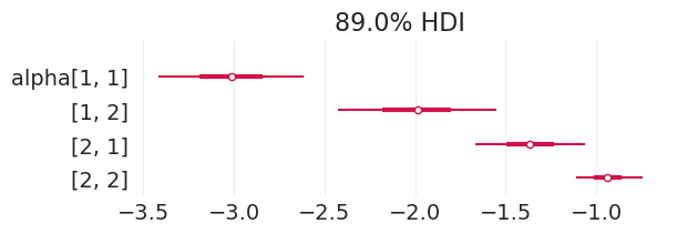
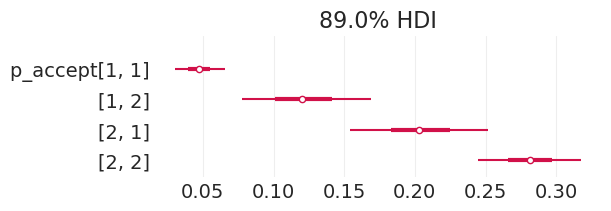
为了比较,这里是基本事实的有偏录取率,我们能够基本恢复
# Department x Gender
BIASED_ACCEPTANCE_RATES
array([[0.05, 0.1 ],
       [0.2 , 0.3 ]])
将直接效应模型拟合到无偏模拟招生数据#
direct_effect_model_simulated_unbiased, direct_effect_inference_simulated_unbiased = (
    fit_direct_effect_model_admissions(SIMULATED_UNBIASED_ADMISSIONS)
)
Initializing NUTS using jitter+adapt_diag...
Multiprocess sampling (4 chains in 4 jobs)
NUTS: [alpha]
Sampling 4 chains for 1_000 tune and 1_000 draw iterations (4_000 + 4_000 draws total) took 1 seconds.
plot_admissions_model_posterior(direct_effect_inference_simulated_unbiased)
| 均值 | 标准差 | HDI_3% | HDI_97% | MCSE_均值 | MCSE_标准差 | ESS_批量 | ESS_尾部 | R_hat | |
|---|---|---|---|---|---|---|---|---|---|
| alpha[1, 1] | -2.155 | 0.175 | -2.460 | -1.805 | 0.002 | 0.002 | 5264.0 | 3200.0 | 1.0 |
| alpha[1, 2] | -2.276 | 0.313 | -2.901 | -1.722 | 0.004 | 0.003 | 5684.0 | 2986.0 | 1.0 |
| alpha[2, 1] | -0.618 | 0.161 | -0.919 | -0.322 | 0.002 | 0.001 | 7013.0 | 3158.0 | 1.0 |
| alpha[2, 2] | -0.898 | 0.114 | -1.114 | -0.684 | 0.001 | 0.001 | 6859.0 | 3242.0 | 1.0 |
| p_accept[1, 1] | 0.105 | 0.016 | 0.076 | 0.136 | 0.000 | 0.000 | 5264.0 | 3200.0 | 1.0 |
| p_accept[1, 2] | 0.096 | 0.027 | 0.050 | 0.148 | 0.000 | 0.000 | 5684.0 | 2986.0 | 1.0 |
| p_accept[2, 1] | 0.351 | 0.036 | 0.284 | 0.419 | 0.000 | 0.000 | 7013.0 | 3158.0 | 1.0 |
| p_accept[2, 2] | 0.290 | 0.023 | 0.243 | 0.331 | 0.000 | 0.000 | 6859.0 | 3242.0 | 1.0 |
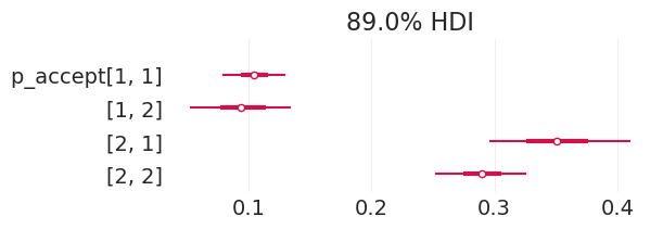
为了比较,这里是基本事实的无偏录取率,我们能够恢复
# Department x Gender
UNBIASED_ACCEPTANCE_RATES
array([[0.1, 0.1],
       [0.3, 0.3]])
4. 分析加州大学伯克利分校的招生数据#
计数数据集回顾#
我们将使用这些计数数据来建模性别/院系录取率的对数几率
请注意,我们将使用二项回归,它等效于伯努利回归,但对聚合计数进行运算,而不是对单个二元试验进行运算
上面的示例实际上是作为二项回归实现的,以便我们可以重用代码并演示一般的分析模式
无论哪种方式,您都将使用这两种方法获得相同的推断
ADMISSIONS
| 院系 | 申请者性别 | 录取 | 拒绝 | 申请数 | |
|---|---|---|---|---|---|
| 1 | A | 男性 | 512 | 313 | 825 |
| 2 | A | 女性 | 89 | 19 | 108 |
| 3 | B | 男性 | 353 | 207 | 560 |
| 4 | B | 女性 | 17 | 8 | 25 |
| 5 | C | 男性 | 120 | 205 | 325 |
| 6 | C | 女性 | 202 | 391 | 593 |
| 7 | D | 男性 | 138 | 279 | 417 |
| 8 | D | 女性 | 131 | 244 | 375 |
| 9 | E | 男性 | 53 | 138 | 191 |
| 10 | E | 女性 | 94 | 299 | 393 |
| 11 | F | 男性 | 22 | 351 | 373 |
| 12 | F | 女性 | 24 | 317 | 341 |
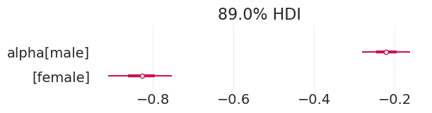
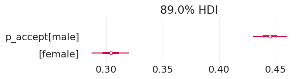
将总效应模型拟合到加州大学伯克利分校的招生数据#
不要忘记查看诊断结果,我们在这里将跳过
total_effect_model, total_effect_inference = fit_total_effect_model_admissions(ADMISSIONS)
Initializing NUTS using jitter+adapt_diag...
Multiprocess sampling (4 chains in 4 jobs)
NUTS: [alpha]
Sampling 4 chains for 1_000 tune and 1_000 draw iterations (4_000 + 4_000 draws total) took 1 seconds.
plot_admissions_model_posterior(total_effect_inference, figsize=(6, 1.5))
| 均值 | 标准差 | HDI_3% | HDI_97% | MCSE_均值 | MCSE_标准差 | ESS_批量 | ESS_尾部 | R_hat | |
|---|---|---|---|---|---|---|---|---|---|
| alpha[男性] | -0.221 | 0.038 | -0.294 | -0.151 | 0.001 | 0.000 | 4202.0 | 2936.0 | 1.0 |
| alpha[女性] | -0.828 | 0.050 | -0.917 | -0.732 | 0.001 | 0.001 | 3905.0 | 2831.0 | 1.0 |
| p_accept[男性] | 0.445 | 0.009 | 0.427 | 0.462 | 0.000 | 0.000 | 4202.0 | 2936.0 | 1.0 |
| p_accept[女性] | 0.304 | 0.011 | 0.286 | 0.325 | 0.000 | 0.000 | 3905.0 | 2831.0 | 1.0 |
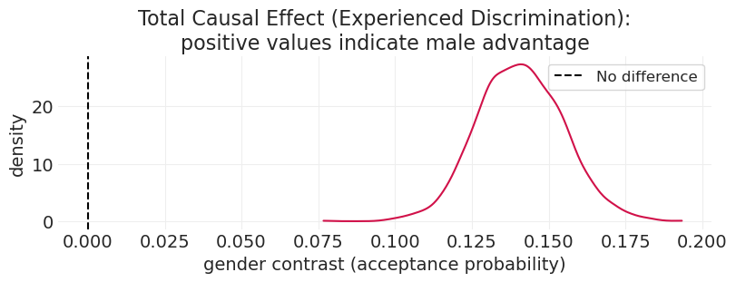
总因果效应#
# Total Causal Effect
female_p_accept = total_effect_inference.posterior["p_accept"].sel(gender="female")
male_p_accept = total_effect_inference.posterior["p_accept"].sel(gender="male")
contrast = male_p_accept - female_p_accept

plt.subplots(figsize=(8, 3))
az.plot_dist(contrast)
plt.axvline(0, linestyle="--", color="black", label="No difference")
plt.xlabel("gender contrast (acceptance probability)")
plt.ylabel("density")
plt.title(
    "Total Causal Effect (Experienced Discrimination):\npositive values indicate male advantage"
)
plt.legend();
将直接效应模型拟合到加州大学伯克利分校的招生数据#
direct_effect_model, direct_effect_inference = fit_direct_effect_model_admissions(ADMISSIONS)
Initializing NUTS using jitter+adapt_diag...
Multiprocess sampling (4 chains in 4 jobs)
NUTS: [alpha]
Sampling 4 chains for 1_000 tune and 1_000 draw iterations (4_000 + 4_000 draws total) took 1 seconds.
plot_admissions_model_posterior(direct_effect_inference, figsize=(6, 3))
| 均值 | 标准差 | HDI_3% | HDI_97% | MCSE_均值 | MCSE_标准差 | ESS_批量 | ESS_尾部 | R_hat | |
|---|---|---|---|---|---|---|---|---|---|
| alpha[A, 男性] | 0.490 | 0.072 | 0.353 | 0.620 | 0.001 | 0.001 | 5850.0 | 3067.0 | 1.0 |
| alpha[A, 女性] | 1.474 | 0.243 | 1.029 | 1.937 | 0.003 | 0.002 | 5579.0 | 2964.0 | 1.0 |
| alpha[B, 男性] | 0.531 | 0.087 | 0.377 | 0.703 | 0.001 | 0.001 | 5106.0 | 2554.0 | 1.0 |
| alpha[B, 女性] | 0.657 | 0.395 | -0.075 | 1.387 | 0.005 | 0.004 | 6701.0 | 3242.0 | 1.0 |
| alpha[C, 男性] | -0.532 | 0.115 | -0.743 | -0.310 | 0.001 | 0.001 | 5940.0 | 3091.0 | 1.0 |
| alpha[C, 女性] | -0.660 | 0.086 | -0.831 | -0.506 | 0.001 | 0.001 | 5786.0 | 3051.0 | 1.0 |
| alpha[D, 男性] | -0.698 | 0.102 | -0.892 | -0.513 | 0.001 | 0.001 | 6055.0 | 3004.0 | 1.0 |
| alpha[D, 女性] | -0.618 | 0.108 | -0.828 | -0.425 | 0.001 | 0.001 | 6215.0 | 2943.0 | 1.0 |
| alpha[E, 男性] | -0.935 | 0.158 | -1.239 | -0.645 | 0.002 | 0.002 | 5672.0 | 2865.0 | 1.0 |
| alpha[E, 女性] | -1.146 | 0.119 | -1.364 | -0.928 | 0.002 | 0.001 | 5891.0 | 2814.0 | 1.0 |
| alpha[F, 男性] | -2.667 | 0.205 | -3.057 | -2.291 | 0.003 | 0.002 | 5224.0 | 2612.0 | 1.0 |
| alpha[F, 女性] | -2.499 | 0.195 | -2.863 | -2.131 | 0.003 | 0.002 | 6109.0 | 3036.0 | 1.0 |
| p_accept[A, 男性] | 0.620 | 0.017 | 0.587 | 0.650 | 0.000 | 0.000 | 5850.0 | 3067.0 | 1.0 |
| p_accept[A, 女性] | 0.811 | 0.037 | 0.742 | 0.878 | 0.000 | 0.000 | 5579.0 | 2964.0 | 1.0 |
| p_accept[B, 男性] | 0.629 | 0.020 | 0.595 | 0.670 | 0.000 | 0.000 | 5106.0 | 2554.0 | 1.0 |
| p_accept[B, 女性] | 0.653 | 0.086 | 0.488 | 0.805 | 0.001 | 0.001 | 6701.0 | 3242.0 | 1.0 |
| p_accept[C, 男性] | 0.370 | 0.027 | 0.322 | 0.423 | 0.000 | 0.000 | 5940.0 | 3091.0 | 1.0 |
| p_accept[C, 女性] | 0.341 | 0.019 | 0.303 | 0.376 | 0.000 | 0.000 | 5786.0 | 3051.0 | 1.0 |
| p_accept[D, 男性] | 0.333 | 0.023 | 0.291 | 0.374 | 0.000 | 0.000 | 6055.0 | 3004.0 | 1.0 |
| p_accept[D, 女性] | 0.351 | 0.025 | 0.304 | 0.395 | 0.000 | 0.000 | 6215.0 | 2943.0 | 1.0 |
| p_accept[E, 男性] | 0.283 | 0.032 | 0.222 | 0.341 | 0.000 | 0.000 | 5672.0 | 2865.0 | 1.0 |
| p_accept[E, 女性] | 0.242 | 0.022 | 0.204 | 0.283 | 0.000 | 0.000 | 5891.0 | 2814.0 | 1.0 |
| p_accept[F, 男性] | 0.066 | 0.012 | 0.043 | 0.089 | 0.000 | 0.000 | 5224.0 | 2612.0 | 1.0 |
| p_accept[F, 女性] | 0.077 | 0.014 | 0.052 | 0.103 | 0.000 | 0.000 | 6109.0 | 3036.0 | 1.0 |
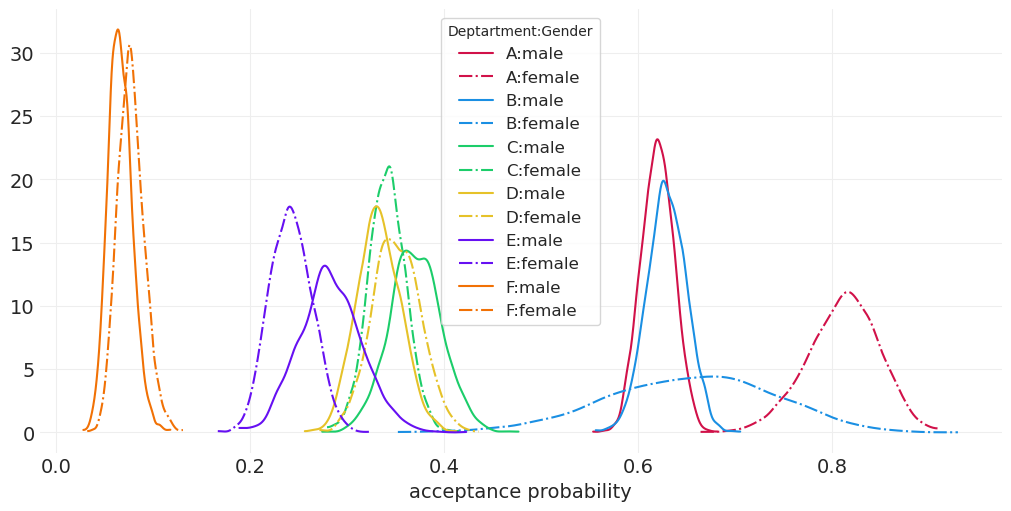
# Fancier plot of department/gender acceptance probability distributions
_, ax = plt.subplots(figsize=(10, 5))
for ii, dept in enumerate(ADMISSIONS.dept.unique()):
    color = f"C{ii}"
    for gend in ADMISSIONS["applicant.gender"].unique():
        label = f"{dept}:{gend}"
        linestyle = "-." if gend == "female" else "-"
        post = direct_effect_inference.posterior["p_accept"].sel(department=dept, gender=gend)
        az.plot_dist(post, label=label, color=color, plot_kwargs={"linestyle": linestyle})
plt.xlabel("acceptance probability")
plt.legend(title="Deptartment:Gender");
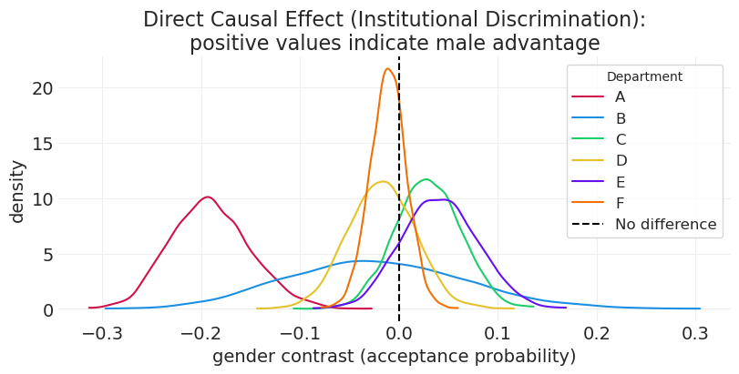
直接因果效应#
# Direct Causal Effect
_, ax = plt.subplots(figsize=(8, 4))

for ii, dept in enumerate(ADMISSIONS.dept.unique()):
    color = f"C{ii}"
    label = f"{dept}"

    female_p_accept = direct_effect_inference.posterior["p_accept"].sel(
        gender="female", department=dept
    )
    male_p_accept = direct_effect_inference.posterior["p_accept"].sel(
        gender="male", department=dept
    )

    contrast = male_p_accept - female_p_accept
    az.plot_dist(contrast, color=color, label=label)

plt.xlabel("gender contrast (acceptance probability)")
plt.ylabel("density")
plt.title(
    "Direct Causal Effect (Institutional Discrimination):\npositive values indicate male advantage"
)
plt.axvline(0, linestyle="--", color="black", label="No difference")
plt.legend(title="Department");
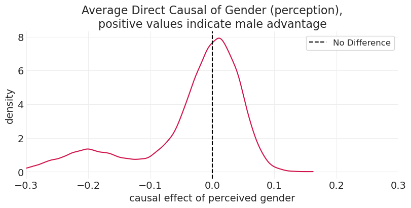
平均直接效应#
性别的因果效应 在各院系之间平均 (边缘化)
取决于每个院系的申请分布
这很容易作为模拟来完成
后分层#
为目标人群重新加权估计值
允许我们将从一所大学拟合的模型应用于估计另一所具有不同院系分布的大学的因果影响
在这里,我们使用经验分布来重新加权估计值
# Use the empirical distribution of departments -- we'd update this for a different university
applications_per_dept = ADMISSIONS.groupby("dept").sum()["applications"].values
total_applications = applications_per_dept.sum()
department_weight = applications_per_dept / total_applications

female_alpha = direct_effect_inference.posterior.sel(gender="female")["alpha"]
male_alpha = direct_effect_inference.posterior.sel(gender="male")["alpha"]

weighted_female_alpha = female_alpha * department_weight
weighed_male_alpha = male_alpha * department_weight

contrast = weighed_male_alpha - weighted_female_alpha

_, ax = plt.subplots(figsize=(8, 4))
az.plot_dist(contrast)

plt.axvline(0, linestyle="--", color="k", label="No Difference")
plt.xlabel("causal effect of perceived gender")
plt.ylabel("density")
plt.title("Average Direct Causal of Gender (perception),\npositive values indicate male advantage")
plt.xlim([-0.3, 0.3])
plt.legend();
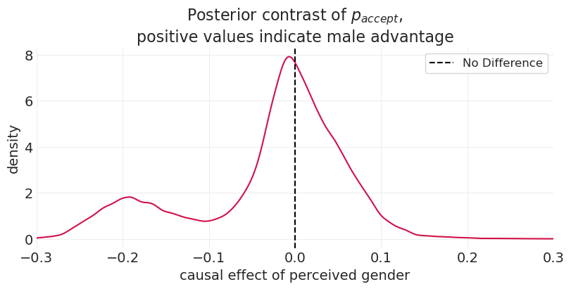
为了验证平均过程,我们可以查看来自后验的 p_accept 样本的对比,这提供了类似的结果。但是,查看后验显然不适用于对样本外大学进行预测。
direct_posterior = direct_effect_inference.posterior

# Select by gender; note: p_accept already has link function applied
female_posterior = direct_posterior.sel(gender="female")[
    "p_accept"
]  # shape: (chain x draw x department)
male_posterior = direct_posterior.sel(gender="male")[
    "p_accept"
]  # shape: (chain x draw x department)
contrast = male_posterior - female_posterior  # shape: (chain x draw x department)

_, ax = plt.subplots(figsize=(8, 4))
# marginalize / collapse the contrast across all departments
az.plot_dist(contrast)
plt.axvline(0, linestyle="--", color="k", label="No Difference")
plt.xlim([-0.3, 0.3])
plt.xlabel("causal effect of perceived gender")
plt.ylabel("density")
plt.title("Posterior contrast of $p_{accept}$,\npositive values indicate male advantage")
plt.legend();
歧视?#
很难说
巨大的结构性影响
申请人的分布可能是由于歧视造成的
混淆因素很可能存在
奖励:生存分析#
计数通常建模为事件发生时间(即指数分布或伽玛分布)——目标是估计事件发生率
很棘手,因为忽略 删失数据 可能会导致推断错误
左删失:我们不知道计时器何时开始
右删失:观察期在事件发生之前结束
示例:奥斯汀猫咪收养#
2 万只猫
事件:被收养 (1) 或未被收养 (0)
删失机制
在被收养前死亡
逃跑
尚未被收养
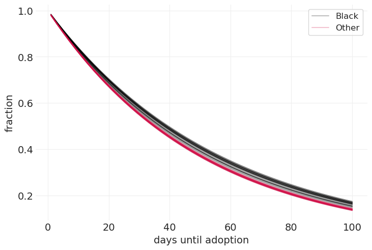
目标:确定黑色猫咪的收养率是否低于非黑色猫咪。
CATS = utils.load_data("AustinCats")
CATS.head()
| ID | 事件发生天数 | 外出日期 | 外出事件 | 进入日期 | 进入事件 | 品种 | 颜色 | 收养年龄 | |
|---|---|---|---|---|---|---|---|---|---|
| 0 | A730601 | 1 | 2016 年 7 月 8 日 上午 09:00:00 | 转移 | 2016 年 7 月 7 日 下午 12:11:00 | 流浪 | 家猫短毛混血 | 蓝色虎斑 | 7 |
| 1 | A679549 | 25 | 2014 年 6 月 16 日 下午 01:54:00 | 转移 | 2014 年 5 月 22 日 下午 03:43:00 | 流浪 | 家猫短毛混血 | 黑色/白色 | 1 |
| 2 | A683656 | 4 | 2014 年 7 月 17 日 下午 04:57:00 | 收养 | 2014 年 7 月 13 日 下午 01:20:00 | 流浪 | 雪鞋猫混血 | 山猫色重点色 | 2 |
| 3 | A709749 | 41 | 2015 年 9 月 22 日 下午 12:49:00 | 转移 | 2015 年 8 月 12 日 下午 06:29:00 | 流浪 | 家猫短毛混血 | 玳瑁色 | 12 |
| 4 | A733551 | 9 | 2016 年 9 月 1 日 上午 12:00:00 | 转移 | 2016 年 8 月 23 日 下午 02:35:00 | 流浪 | 家猫短毛混血 | 棕色虎斑/白色 | 1 |
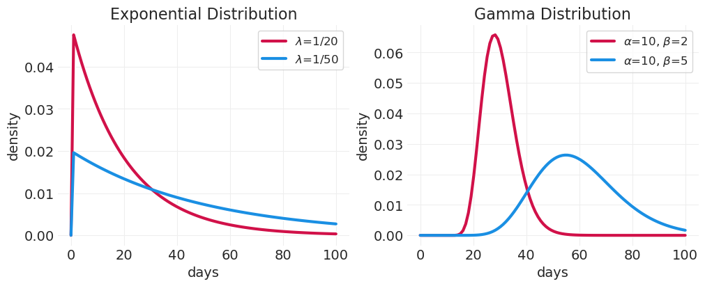
建模结果变量:days_to_event#
建模事件发生时间的两种常用分布
指数分布:
两者中较简单的一种(单参数)
假设恒定速率
在具有相同平均速率的非负连续分布集中,熵最大分布。
假设在事件发生(机器故障)之前发生一件事情(例如,零件故障)
伽玛分布
两者中更复杂的一种(两个参数)
在具有相同均值和平均对数的分布集中,熵最大分布。
假设在事件发生(机器故障)之前发生多件事情(例如,零件故障)
_, axs = plt.subplots(1, 2, figsize=(10, 4))

days = np.linspace(0, 100, 100)

plt.sca(axs[0])
for scale in [20, 50]:
    expon = stats.expon(loc=0.01, scale=scale)
    utils.plot_line(days, expon.pdf(days), label=f"$\\lambda$=1/{scale}")
plt.xlabel("days")
plt.ylabel("density")
plt.legend()
plt.title("Exponential Distribution")


plt.sca(axs[1])
N = 8
alpha = 10
for scale in [2, 5]:
    gamma = stats.gamma(a=10, loc=alpha, scale=scale)
    utils.plot_line(days, gamma.pdf(days), label=f"$\\alpha$={alpha}, $\\beta$={scale}")
plt.xlabel("days")
plt.ylabel("density")
plt.legend()
plt.title("Gamma Distribution");
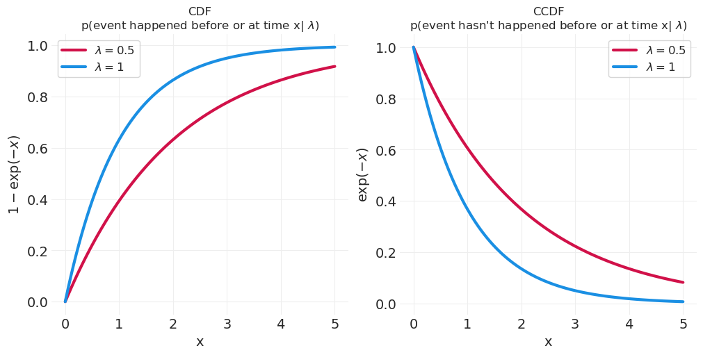
删失和非删失观测#
观测数据使用累积分布;即,事件在时间 x 之前发生的概率
未观测到的(删失)数据则需要 CDF 的互补;即,事件尚未发生的概率。
xs = np.linspace(0, 5, 100)
_, axs = plt.subplots(1, 2, figsize=(10, 5))
plt.sca(axs[0])
cdfs = {}
for lambda_ in [0.5, 1]:
    cdfs[lambda_] = ys = 1 - np.exp(-lambda_ * xs)
    utils.plot_line(xs, ys, label=f"$\\lambda={lambda_}$")

plt.xlabel("x")
plt.ylabel("$1 - \\exp(-x)$")
plt.legend()
plt.title("CDF\np(event happened before or at time x| $\\lambda$)", fontsize=12)

plt.sca(axs[1])
for lambda_ in [0.5, 1]:
    ys = 1 - cdfs[lambda_]
    utils.plot_line(xs, ys, label=f"$\\lambda={lambda_}$")

plt.xlabel("x")
plt.ylabel("$\\exp(-x)$")
plt.legend()
plt.title("CCDF\np(event hasn't happened before or at time x| $\\lambda$)", fontsize=12);
统计模型#
\(D_i | A_i = 1\) - 观测到的收养
\(D_i | A_i = 1\) - 尚未观测到的收养
\(\alpha_{\text{猫咪颜色}[i]}\) 每种猫咪颜色的对数平均收养时间
\(\log \mu_i\) – 链接函数确保 \(\alpha\) 为正数
\(\lambda_i = \frac{1}{\mu_i}\) 简化了估计平均 收养时间
为 \(\alpha\) 找到合理的超参数#
我们需要确定指数先验均值参数 \(\gamma\) 的合理数据。为此,我们将查看收养时间的经验分布
# determine reasonable prior for alpha
plt.subplots(figsize=(6, 3))
CATS[CATS.out_event == "Adoption"].days_to_event.hist(bins=100)
plt.xlim([0, 500]);
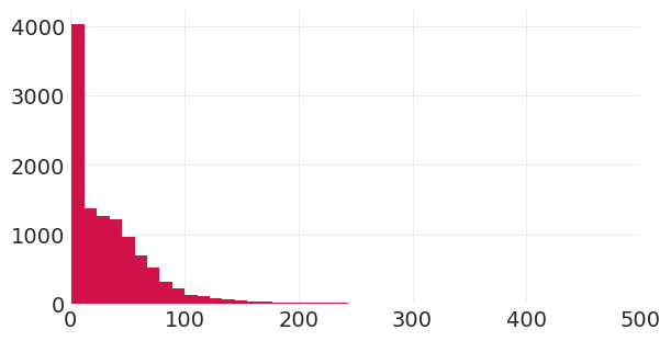
使用上面的经验直方图,我们看到大部分概率质量在 0 到 200 之间,因此让我们使用 50 作为预期等待时间。
CAT_COLOR_ID, CAT_COLOR = pd.factorize(CATS.color.apply(lambda x: "Other" if x != "Black" else x))
ADOPTED_ID, ADOPTED = pd.factorize(
    CATS.out_event.apply(lambda x: "Other" if x != "Adoption" else "Adopted")
)
DAYS_TO_ADOPTION = CATS.days_to_event.values.astype(float)
LAMBDA = 50

with pm.Model(coords={"cat_color": CAT_COLOR}) as adoption_model:

    # Censoring
    right_censoring = DAYS_TO_ADOPTION.copy()
    right_censoring[ADOPTED_ID == 0] = DAYS_TO_ADOPTION.max()

    # Priors
    gamma = 1 / LAMBDA
    alpha = pm.Exponential("alpha", gamma, dims="cat_color")

    # Likelihood
    log_adoption_rate = 1 / alpha[CAT_COLOR_ID]
    pm.Censored(
        "adopted",
        pm.Exponential.dist(lam=log_adoption_rate),
        lower=None,
        upper=right_censoring,
        observed=DAYS_TO_ADOPTION,
    )
    adoption_inference = pm.sample()
Initializing NUTS using jitter+adapt_diag...
Multiprocess sampling (4 chains in 4 jobs)
NUTS: [alpha]
Sampling 4 chains for 1_000 tune and 1_000 draw iterations (4_000 + 4_000 draws total) took 14 seconds.
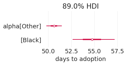
可怜的黑色小猫 🐈⬛#
看来黑色猫咪确实需要更长的时间才能被收养。
后验摘要#
_, ax = plt.subplots(figsize=(4, 2))
az.plot_forest(adoption_inference, var_names=["alpha"], combined=True, hdi_prob=0.89, ax=ax)
plt.xlabel("days to adoption");
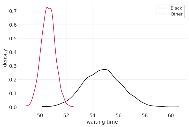
后验分布#
for ii, cat_color in enumerate(["Black", "Other"]):
    color = "black" if cat_color == "Black" else "C0"
    posterior_alpha = adoption_inference.posterior.sel(cat_color=cat_color)["alpha"]
    az.plot_dist(posterior_alpha, color=color, label=cat_color)
plt.xlabel("waiting time")
plt.ylabel("density")
plt.legend();
days_until_adoption_ = np.linspace(1, 100)
n_posterior_samples = 25

for cat_color in ["Black", "Other"]:
    color = "black" if cat_color == "Black" else "C0"
    posterior = adoption_inference.posterior.sel(cat_color=cat_color)
    alpha_samples = posterior.alpha.sel(chain=0)[:n_posterior_samples].values
    for ii, alpha in enumerate(alpha_samples):
        label = cat_color if ii == 0 else None
        plt.plot(
            days_until_adoption_,
            np.exp(-days_until_adoption_ / alpha),
            color=color,
            alpha=0.25,
            label=label,
        )

plt.xlabel("days until adoption")
plt.ylabel("fraction")
plt.legend();
许可声明#
此示例库中的所有笔记本均根据 MIT 许可证 提供,该许可证允许修改和再分发用于任何用途,前提是保留版权和许可声明。
引用 PyMC 示例#
要引用此笔记本,请使用 Zenodo 为 pymc-examples 存储库提供的 DOI。
重要提示
许多笔记本改编自其他来源:博客、书籍……在这种情况下,您也应该引用原始来源。
另请记住引用您的代码使用的相关库。
这是一个 bibtex 中的引用模板
@incollection{citekey,
  author    = "<notebook authors, see above>",
  title     = "<notebook title>",
  editor    = "PyMC Team",
  booktitle = "PyMC examples",
  doi       = "10.5281/zenodo.5654871"
}
渲染后可能看起来像