


分叉数据花园#
此笔记本是 PyMC 移植的 Statistical Rethinking 2023 Richard McElreath 讲座系列的一部分。
视频 - 讲座 10 - 计数和隐藏的混淆因素# 讲座 10 - 计数和隐藏的混淆因素
# Ignore warnings
import warnings

import arviz as az
import numpy as np
import pandas as pd
import pymc as pm
import statsmodels.formula.api as smf
import utils as utils
import xarray as xr

from matplotlib import pyplot as plt
from matplotlib import style
from scipy import stats as stats

warnings.filterwarnings("ignore")

# Set matplotlib style
STYLE = "statistical-rethinking-2023.mplstyle"
style.use(STYLE)
重新审视广义线性模型#
期望值是参数加性组合的某个函数
该函数倾向于与数据似然分布相关联 – 例如,正态分布的恒等函数(线性回归)或伯努利/二项分布的对数几率(逻辑回归)
预测变量的均匀变化通常与结果的均匀变化无关
预测变量相互作用 – 系数的因果解释(在最简单的模型之外)充满了误导性的结论
混淆的录取#
utils.draw_causal_graph(
    edge_list=[("G", "D"), ("G", "A"), ("D", "A"), ("u", "D"), ("u", "A")],
    node_props={
        "u": {"style": "dashed", "label": "Ability, u"},
        "G": {"label": "Gender, G"},
        "D": {"label": "Department, D"},
        "A": {"label": "Admission, A"},
        "unobserved": {"style": "dashed"},
    },
)

我们估计了性别对录取率的直接和总效应,以便识别招生中不同形式的性别歧视
然而,变量之间不存在未观察到的混淆因素是难以置信的,
例如,申请人能力可能会将院系与录取率联系起来
影响哪些学生申请每个院系(能力越强,院系申请偏差越大)
也影响基线录取率(能力越强,录取率越高)
生成模拟#
np.random.seed(1)

# Number of applicants
n_samples = 2000

# Gender equally likely
G = np.random.choice([0, 1], size=n_samples, replace=True)

# Unobserved Ability -- 10% have High, everyone else is Average
u = stats.bernoulli.rvs(p=0.1, size=n_samples)

# Choice of department
# G0 applies to D0 with 75% probability else D1 with 1% or 0% based on ability
D = stats.bernoulli.rvs(p=np.where(G == 0, u * 1.0, 0.75))

# Ability-based acceptance rates (ability x dept x gender)
p_u0_dg = np.array([[0.1, 0.1], [0.1, 0.3]])
p_u1_dg = np.array([[0.3, 0.5], [0.3, 0.5]])
p_udg = np.array([p_u0_dg, p_u1_dg])
print("Acceptance Probabilities\n(ability x dept x gender):\n\n", p_udg)

# Simulate acceptance
p = p_udg[u, D, G]
A = stats.bernoulli.rvs(p=p)
Acceptance Probabilities
(ability x dept x gender):

 [[[0.1 0.1]
  [0.1 0.3]]

 [[0.3 0.5]
  [0.3 0.5]]]
总效应估计器#
utils.draw_causal_graph(
    edge_list=[("G", "D"), ("G", "A"), ("D", "A"), ("u", "D"), ("u", "A")],
    node_props={
        "u": {"style": "dashed", "label": "Ability, u"},
        "G": {"label": "Gender, G"},
        "D": {"label": "Department, D"},
        "A": {"label": "Admission, A"},
        "unobserved": {"style": "dashed"},
    },
    edge_props={
        ("G", "A"): {"color": "red"},
        ("G", "D"): {"color": "red"},
        ("D", "A"): {"color": "red"},
    },
)

估计总效应不需要调整集,仅在 GLM 中对性别建模
拟合总效应模型#
# Define coordinates
GENDER_ID, GENDER = pd.factorize(["G2" if g else "G1" for g in G], sort=True)
DEPTARTMENT_ID, DEPARTMENT = pd.factorize(["D2" if d else "D1" for d in D], sort=True)
# Gender-only model
with pm.Model(coords={"gender": GENDER}) as total_effect_admissions_model:
    alpha = pm.Normal("alpha", 0, 1, dims="gender")

    # Likelihood
    p = pm.math.invlogit(alpha[GENDER_ID])
    pm.Bernoulli("admitted", p=p, observed=A)

    # Record the probability param for simpler reporting
    pm.Deterministic("p_admit", pm.math.invlogit(alpha), dims="gender")

    total_effect_admissions_inference = pm.sample()
Initializing NUTS using jitter+adapt_diag...
Multiprocess sampling (4 chains in 4 jobs)
NUTS: [alpha]
Sampling 4 chains for 1_000 tune and 1_000 draw iterations (4_000 + 4_000 draws total) took 1 seconds.
pm.model_to_graphviz(total_effect_admissions_model)

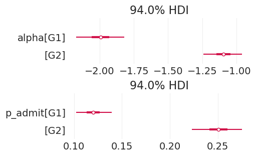
总结总效应估计#
def summarize_posterior(inference, figsize=(5, 3)):
    """Helper function for displaying model fits"""
    _, axs = plt.subplots(2, 1, figsize=figsize)
    az.plot_forest(inference, var_names="alpha", combined=True, ax=axs[0])
    az.plot_forest(inference, var_names="p_admit", combined=True, ax=axs[1])
    return az.summary(inference, var_names=["alpha", "p_admit"])
summarize_posterior(total_effect_admissions_inference)
| 均值 | 标准差 | hdi_3% | hdi_97% | mcse_mean | mcse_sd | ess_bulk | ess_tail | r_hat | |
|---|---|---|---|---|---|---|---|---|---|
| alpha[G1] | -1.994 | 0.095 | -2.171 | -1.820 | 0.002 | 0.001 | 3847.0 | 3137.0 | 1.0 |
| alpha[G2] | -1.095 | 0.075 | -1.240 | -0.958 | 0.001 | 0.001 | 4479.0 | 2904.0 | 1.0 |
| p_admit[G1] | 0.120 | 0.010 | 0.102 | 0.139 | 0.000 | 0.000 | 3847.0 | 3137.0 | 1.0 |
| p_admit[G2] | 0.251 | 0.014 | 0.223 | 0.275 | 0.000 | 0.000 | 4479.0 | 2904.0 | 1.0 |
直接效应估计器(现在由于共同的能力原因而混淆)#
utils.draw_causal_graph(
    edge_list=[("G", "D"), ("G", "A"), ("D", "A"), ("u", "D"), ("u", "A")],
    node_props={
        "u": {"style": "dashed", "label": "Ability, u"},
        "G": {"label": "Gender, G"},
        "D": {"label": "Department, D", "style": "filled"},
        "A": {"label": "Admission, A"},
        "Direct effect\nadjustment set": {"style": "filled"},
        "unobserved": {"style": "dashed"},
    },
    edge_props={
        ("G", "A"): {"color": "red"},
        ("G", "D"): {"color": "blue"},
        ("u", "D"): {"color": "blue"},
        ("u", "A"): {"color": "blue"},
    },
)

估计直接效应包括调整集中的院系
然而,按院系(对撞机)分层 打开了通过未观察到的能力 u 的混淆因素后门路径
拟合(混淆的)直接效应模型#
with pm.Model(
    coords={"gender": GENDER, "department": DEPARTMENT}
) as direct_effect_admissions_model:
    # Prior
    alpha = pm.Normal("alpha", 0, 1, dims=["department", "gender"])

    # Likelihood
    p = pm.math.invlogit(alpha[DEPTARTMENT_ID, GENDER_ID])
    pm.Bernoulli("admitted", p=p, observed=A)

    # Record the acceptance probability parameter for reporting
    pm.Deterministic("p_admit", pm.math.invlogit(alpha), dims=["department", "gender"])

    direct_effect_admissions_inference = pm.sample(tune=2000)

pm.model_to_graphviz(direct_effect_admissions_model)
Initializing NUTS using jitter+adapt_diag...
Multiprocess sampling (4 chains in 4 jobs)
NUTS: [alpha]
Sampling 4 chains for 2_000 tune and 1_000 draw iterations (8_000 + 4_000 draws total) took 2 seconds.

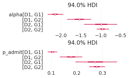
总结(混淆的)直接效应估计#
summarize_posterior(direct_effect_admissions_inference)
| 均值 | 标准差 | hdi_3% | hdi_97% | mcse_mean | mcse_sd | ess_bulk | ess_tail | r_hat | |
|---|---|---|---|---|---|---|---|---|---|
| alpha[D1, G1] | -2.147 | 0.105 | -2.330 | -1.935 | 0.001 | 0.001 | 6328.0 | 3017.0 | 1.0 |
| alpha[D1, G2] | -1.539 | 0.165 | -1.843 | -1.239 | 0.002 | 0.001 | 8058.0 | 3016.0 | 1.0 |
| alpha[D2, G1] | -0.992 | 0.223 | -1.417 | -0.586 | 0.003 | 0.002 | 7155.0 | 3095.0 | 1.0 |
| alpha[D2, G2] | -0.957 | 0.083 | -1.100 | -0.790 | 0.001 | 0.001 | 7375.0 | 3234.0 | 1.0 |
| p_admit[D1, G1] | 0.105 | 0.010 | 0.087 | 0.123 | 0.000 | 0.000 | 6328.0 | 3017.0 | 1.0 |
| p_admit[D1, G2] | 0.178 | 0.024 | 0.134 | 0.221 | 0.000 | 0.000 | 8058.0 | 3016.0 | 1.0 |
| p_admit[D2, G1] | 0.273 | 0.044 | 0.195 | 0.357 | 0.001 | 0.000 | 7155.0 | 3095.0 | 1.0 |
| p_admit[D2, G2] | 0.278 | 0.017 | 0.248 | 0.310 | 0.000 | 0.000 | 7375.0 | 3234.0 | 1.0 |
解释(混淆的)直接效应估计#
def plot_department_gender_admissions(inference, title):
plt.subplots(figsize=(8, 3))
for ii, dept in enumerate(["D1", "D2"]):
for jj, gend in enumerate(["G1", "G2"]):
# note inverse link function applied
post = inference.posterior
post_p_accept = post.sel(department=dept, gender=gend)["p_admit"]
label = f'{dept}({"biased" if ii else "unbiased"})-G{jj+1}'
color = f"C{np.abs(ii - 1)}" # flip colorscale to match lecture
linestyle = "--" if jj else "-"
az.plot_dist(
post_p_accept,
color=color,
label=label,
plot_kwargs=dict(linestyle=linestyle),
)
plt.xlim([0, 0.5])
plt.xlabel("admission probability")
plt.ylabel("density")
plt.title(title)
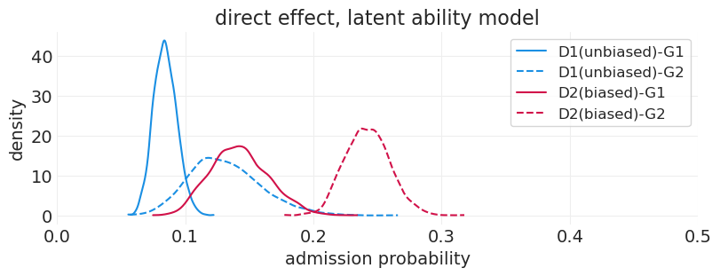
plot_department_gender_admissions(
direct_effect_admissions_inference, "direct effect, confounded model"
)
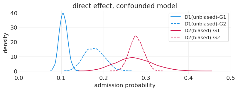
解释混淆的直接效应模型#
在 D1 中,G1 似乎处于不利地位,录取率较低。但是,我们知道这不是真的。发生的情况是,所有能力较高的 G1 申请人都被送到 D2,从而人为地降低了 D1 中 G1 的录取率
我们知道 D2 中存在偏差,但是,我们几乎看不到歧视的证据。这是由于能力较高的 G1 申请人通过具有高于平均水平的录取率来抵消这种偏差
我们可以看到 D2 的 G1 估计值具有更高的方差;这是因为只有 10% 的申请人具有高能力,因此总体而言,申请 D2 的 G1 申请人较少。
你猜对了:对撞机偏差#
这是由于对撞机偏差
按院系分层——院系与性别和能力形成对撞机——打开了一条通过能力到接受的路径。
你不能估计 \(D\) 对 \(G\) 的直接效应
你可以估计总效应
排序可以掩盖或加剧偏差
类比示例:NAS 会员资格和引用次数#
两篇论文
相同数据
发现关于性别及其对美国国家科学院 (NAS) 入选的影响的截然不同的结论
一篇发现女性明显有利
另一篇发现女性明显不利
两个结论怎么可能都是正确的?
utils.draw_causal_graph(
    edge_list=[("G", "C"), ("G", "M"), ("C", "M"), ("q", "C"), ("q", "M")],
    node_props={
        "q": {"style": "dashed", "label": "Researcher quality, q"},
        "G": {"label": "Gender, G"},
        "C": {"label": "Citations, C"},
        "M": {"label": "NAS Member, M"},
        "unobserved": {"style": "dashed"},
    },
)

可能存在潜在的研究人员质量差异
按引用次数分层会打开一个与未观察到的研究人员质量的对撞机偏差。引用次数是后处理变量
引用分层提供误导性结论
例如,如果出版/引用中存在歧视,则一个性别可能会以更高的比率当选,仅仅是因为对于任何引用水平,他们平均都具有更高的质量
没有原因输入,就没有原因输出#
这些论文存在许多缺点
模糊的估计量
不明智的调整集
需要比提出的更强的假设
对撞机偏差可能会对政策设计产生不良影响
定性数据在这些情况下可能很有用
敏感性分析:建模潜在能力混淆变量#
我们无法衡量的东西有什么影响?
类似于直接效应情景
估计直接效应包括调整集中的院系
然而,按院系(对撞机)分层 打开了通过未观察到的能力 u 的混淆因素后门路径
utils.draw_causal_graph(
    edge_list=[("G", "D"), ("G", "A"), ("D", "A"), ("u", "D"), ("u", "A")],
    node_props={
        "u": {"label": "Ability, u", "style": "dashed"},
        "G": {
            "label": "Gender, G",
        },
        "D": {"label": "Department, D", "style": "filled"},
        "A": {"label": "Admission, A"},
        "Sensitivity analysis\nadjustment set": {"style": "filled"},
        "Modeled as\nrandom variable": {"style": "dashed"},
    },
    edge_props={
        ("G", "A"): {"color": "red"},
        ("G", "D"): {"color": "blue"},
        ("u", "D"): {"color": "green", "label": "gamma", "fontcolor": "green"},
        ("u", "A"): {"color": "green", "label": "beta", "fontcolor": "green"},
    },
)

虽然我们无法直接衡量潜在的混淆因素,但我们可以做的是模拟潜在混淆因素的影响程度。具体来说,我们可以建立一个模拟,在其中创建一个与潜在混淆因素相关的随机变量,然后权衡该混淆因素对生成观察数据的贡献量。
在这个特定示例中,我们可以模拟能力随机变量 \(U \sim \text{Normal}(0, 1)\) 的影响程度,方法是将该变量的线性加权贡献添加到接受的对数几率和选择院系(这是因为在我们的因果图中 u 同时影响 D 和 A)
院系子模型#
接受子模型#
我们 手动设置 \(\beta_{G[i]}\) 和 \(\gamma_{G[i]}\) 的值 以执行模拟
拟合潜在能力模型#
# Gender-specific counterfactual parameters
# Ability confound affects admission rates equally for genders
BETA = np.array([1.0, 1.0])

# Ability confound affects department application differentially
# for genders (as is the case in generative data process)
GAMMA = np.array([1.0, 0.0])

coords = {"gender": GENDER, "department": DEPARTMENT, "obs": np.arange(n_samples)}

with pm.Model(coords=coords) as latent_ability_model:

    # Latent ability variable, one for each applicant
    U = pm.Normal("u", 0, 1, dims="obs")

    # Department application submodel
    delta = pm.Normal("delta", 0, 1, dims="gender")
    q = pm.math.invlogit(delta[GENDER_ID] + GAMMA[GENDER_ID] * U)

    selected_department = pm.Bernoulli("d", p=q, observed=D)

    # Acceptance submodel
    alpha = pm.Normal("alpha", 0, 1, dims=["department", "gender"])
    p = pm.math.invlogit(alpha[GENDER_ID, selected_department] + BETA[GENDER_ID] * U)
    pm.Bernoulli("accepted", p=p, observed=A)

    # Record p(A | D, G) for reporting
    p_admit = pm.Deterministic("p_admit", pm.math.invlogit(alpha), dims=["department", "gender"])

    latent_ability_inference = pm.sample()

pm.model_to_graphviz(latent_ability_model)
Initializing NUTS using jitter+adapt_diag...
Multiprocess sampling (4 chains in 4 jobs)
NUTS: [u, delta, alpha]
Sampling 4 chains for 1_000 tune and 1_000 draw iterations (4_000 + 4_000 draws total) took 10 seconds.

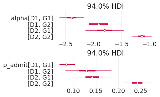
总结潜在能力估计#
summarize_posterior(latent_ability_inference)
| 均值 | 标准差 | hdi_3% | hdi_97% | mcse_mean | mcse_sd | ess_bulk | ess_tail | r_hat | |
|---|---|---|---|---|---|---|---|---|---|
| alpha[D1, G1] | -2.390 | 0.117 | -2.606 | -2.166 | 0.001 | 0.001 | 6488.0 | 2929.0 | 1.0 |
| alpha[D1, G2] | -1.912 | 0.245 | -2.351 | -1.424 | 0.003 | 0.002 | 6028.0 | 3166.0 | 1.0 |
| alpha[D2, G1] | -1.807 | 0.186 | -2.142 | -1.454 | 0.003 | 0.002 | 4981.0 | 3018.0 | 1.0 |
| alpha[D2, G2] | -1.143 | 0.094 | -1.313 | -0.966 | 0.001 | 0.001 | 5004.0 | 2985.0 | 1.0 |
| p_admit[D1, G1] | 0.084 | 0.009 | 0.069 | 0.103 | 0.000 | 0.000 | 6488.0 | 2929.0 | 1.0 |
| p_admit[D1, G2] | 0.131 | 0.028 | 0.082 | 0.185 | 0.000 | 0.000 | 6028.0 | 3166.0 | 1.0 |
| p_admit[D2, G1] | 0.143 | 0.023 | 0.101 | 0.184 | 0.000 | 0.000 | 4981.0 | 3018.0 | 1.0 |
| p_admit[D2, G2] | 0.242 | 0.017 | 0.210 | 0.274 | 0.000 | 0.000 | 5004.0 | 2985.0 | 1.0 |
解释建模混淆因素的效果#
plot_department_gender_admissions(
    direct_effect_admissions_inference, "direct effect, confounded model"
)
plot_department_gender_admissions(latent_ability_inference, "direct effect, latent ability model")
通过添加与数据生成过程一致的敏感性分析,我们能够识别院系 2 中的性别偏见
敏感性分析回顾#
混淆因素确实存在,即使我们无法直接衡量它们 – 不要简单地假装它们不存在
解决问题:我们不知道的事情有什么影响?
SA 介于模拟和分析之间
硬编码我们不知道的东西,让其余的自行发展。
在一定范围内(例如,标准差)改变混淆因素,并显示这种变化如何影响估计值
比假装混淆因素不存在更诚实。
关于参数数量的说明 🤯#
敏感性分析模型有 2006 个自由参数
只有 2000 个观测值
在贝叶斯分析中没什么大不了的
最小样本量为 0,我们只需回退到先验
计数和泊松回归#
Kline & Boyd 海洋技术数据集#
社会的技术复杂性与人口规模有何关系?
估计量:人口规模和接触对工具总数的影响
# Load the data
KLINE = utils.load_data("Kline")
KLINE
| 文化 | 人口 | 接触 | 工具总数 | 平均 TU | |
|---|---|---|---|---|---|
| 0 | 马莱库拉岛 | 1100 | 低 | 13 | 3.2 |
| 1 | 提科皮亚岛 | 1500 | 低 | 22 | 4.7 |
| 2 | 圣克鲁斯岛 | 3600 | 低 | 24 | 4.0 |
| 3 | 雅浦岛 | 4791 | 高 | 43 | 5.0 |
| 4 | 劳群岛斐济 | 7400 | 高 | 33 | 5.0 |
| 5 | 特罗布里恩群岛 | 8000 | 高 | 19 | 4.0 |
| 6 | 楚克群岛 | 9200 | 高 | 40 | 3.8 |
| 7 | 马努斯岛 | 13000 | 低 | 28 | 6.6 |
| 8 | 汤加 | 17500 | 高 | 55 | 5.4 |
| 9 | 夏威夷 | 275000 | 低 | 71 | 6.6 |
概念想法#
创新越多,工具越多
人越多,创新越多
文化之间的接触越多,创新越多
创新(工具)也会随着时间的推移而被遗忘或变得过时
utils.draw_causal_graph(
    edge_list=[
        ("Population", "Innovation"),
        ("Innovation", "Tools Developed"),
        ("Contact Level", "Innovation"),
        ("Tools Developed", "Tool Loss"),
        ("Tool Loss", "Total Tools Observed"),
    ],
    graph_direction="LR",
)

科学模型#
utils.draw_causal_graph(
    edge_list=[("C", "T"), ("L", "T"), ("L", "P"), ("L", "C"), ("P", "C"), ("P", "T")],
    node_props={"L": {"style": "dashed"}, "unobserved": {"style": "dashed"}},
    graph_direction="LR",
)

人口是处理
工具是结果
接触水平调节人口的影响(管道)
位置是未观察到的混淆因素
更好的材料
靠近其他文化
可以支持更大的人口
我们现在忽略
人口对工具的直接效应的调整集
位置,如果可以观察到的话
也按接触分层以研究相互作用
建模工具总数#
工具没有上限 –> 不能使用二项分布
泊松分布接近二项分布,对于大的 \(N\)(接近无穷大)和小的 \(p\)(接近 0)
泊松 GLM#
链接函数是 \(\log(\lambda)\)
逆链接函数是 \(\exp(\alpha + \beta x_i)\)
严格正 \(\lambda\)(由于指数函数)
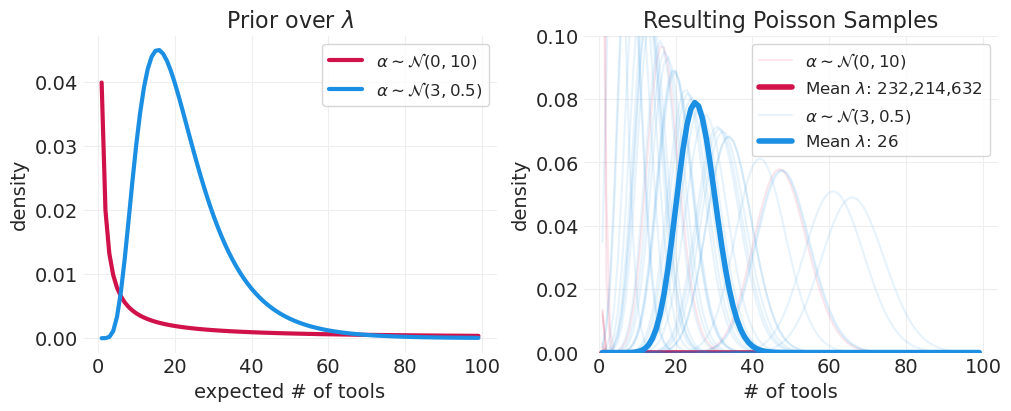
泊松先验#
注意指数缩放,它会产生令人震惊的结果! 通常会导致长尾
更容易移动位置(例如,正态先验的均值),并保持紧密的方差
先验方差通常需要非常紧密,在 0.1 - 0.5 的数量级
np.random.seed(123)
num_tools = np.arange(1, 100)
_, axs = plt.subplots(1, 2, figsize=(10, 4))

plt.sca(axs[0])

normal_alpha_prior_params = [(0, 10), (3, 0.5)]  # flat, centered prior  # offset, tight prior

for prior_mu, prior_sigma in normal_alpha_prior_params:
    # since log(lambda) = alpha, if
    # alpha is Normally distributed, therefore lambda is log-normal
    lambda_prior_dist = stats.lognorm(s=prior_sigma, scale=np.exp(prior_mu))
    label = f"$\\alpha \sim \mathcal{{N}}{prior_mu, prior_sigma}$"
    pdf = lambda_prior_dist.pdf(num_tools)
    plt.plot(num_tools, pdf, label=label, linewidth=3)

plt.xlabel("expected # of tools")
plt.ylabel("density")
plt.legend()
plt.title("Prior over $\\lambda$")

plt.sca(axs[1])

n_prior_samples = 30
for ii, (prior_mu, prior_sigma) in enumerate(normal_alpha_prior_params):

    # Sample lambdas from the prior
    prior_dist = stats.norm(prior_mu, prior_sigma)
    alphas = prior_dist.rvs(n_prior_samples)
    lambdas = np.exp(alphas)
    mean_lambda = lambdas.mean()

    for sample_idx, lambda_ in enumerate(lambdas):
        pmf = stats.poisson(lambda_).pmf(num_tools)

        label = f"$\\alpha \sim \mathcal{{N}}{prior_mu, prior_sigma}$" if sample_idx == 1 else None
        color = f"C{ii}"
        plt.plot(num_tools, pmf, color=color, label=label, alpha=0.1)

    mean_lambda_ = np.exp(alphas).mean()
    pmf = stats.poisson(mean_lambda_).pmf(num_tools)
    plt.plot(
        num_tools,
        pmf,
        color=color,
        label=f"Mean $\\lambda$: {mean_lambda:1,.0f}",
        alpha=1,
        linewidth=4,
    )

plt.xlabel("# of tools")
plt.ylabel("density")
plt.ylim([0, 0.1])
plt.legend()
plt.title("Resulting Poisson Samples");
在混合中添加斜率 \(\log(\lambda_i) = \alpha + \beta x_i\)#
np.random.seed(123)
normal_alpha_prior_params = [(0, 1), (3, 0.5)]  # flat, centered prior  # offset, tight prior

normal_beta_prior_params = [(0, 10), (0, 0.2)]  # flat, centered prior  # tight, centered

n_prior_samples = 10
_, axs = plt.subplots(1, 2, figsize=(10, 4))
xs = np.linspace(-2, 2, 100)[:, None]
for ii, (a_params, b_params) in enumerate(zip(normal_alpha_prior_params, normal_beta_prior_params)):
    plt.sca(axs[ii])
    alpha_prior_samples = stats.norm(*a_params).rvs(n_prior_samples)
    beta_prior_samples = stats.norm(*b_params).rvs(n_prior_samples)
    lambda_samples = np.exp(alpha_prior_samples + xs * beta_prior_samples)

    utils.plot_line(xs, lambda_samples, label=None, color="C0")
    plt.ylim([0, 100])
    plt.title(f"$\\alpha \\sim Normal{a_params}$\n$\\beta \\sim Normal{b_params}$")
    plt.xlabel("x value")
    plt.ylabel("expected count")
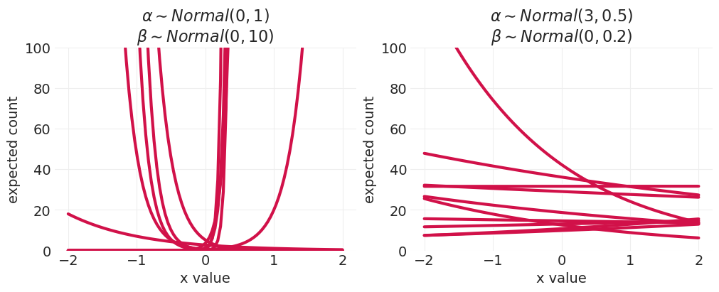
从两种不同类型的先验中提取的预期计数函数
左图:宽先验
右图:紧先验
直接效应估计器#
估计人口 P 对工具数量 T 的直接效应包括接触水平 C 在调整集中,以及位置 L(目前未观察到;我们现在忽略)
utils.draw_causal_graph(
    edge_list=[("L", "C"), ("P", "C"), ("C", "T"), ("L", "T"), ("L", "P"), ("P", "T")],
    node_props={
        "L": {"label": "location, L", "style": "dashed,filled"},
        "C": {"label": "contact, C", "style": "filled"},
        "P": {"label": "population, P"},
        "T": {"label": "number of tools, T"},
        "unobserved": {"style": "dashed"},
        "Direct Effect\nadjustment set": {"style": "filled"},
    },
    edge_props={("P", "T"): {"color": "red"}},
)

比较模型#
我们将估计几个模型,以便练习模型比较
模型 A)一个简单的全局截距泊松 GLM
模型 B)一个泊松 GLM,包括截距和标准化对数人口的参数,这两者都按接触水平分层
模型 A - 全局截距模型#
在这里,我们将工具计数建模为泊松随机变量。泊松率参数是线性模型的指数。在这个线性模型中,我们只包括低或高接触人口的偏移量。
# Set up data and coords
TOOLS = KLINE.total_tools.values.astype(float)
with pm.Model() as global_intercept_model:

    # Prior on global intercept
    alpha = pm.Normal("alpha", 3.0, 0.5)

    # Likelihood
    lam = pm.math.exp(alpha)
    pm.Poisson("tools", lam, observed=TOOLS)

    global_intercept_inference = pm.sample()
    global_intercept_inference = pm.compute_log_likelihood(global_intercept_inference)

pm.model_to_graphviz(global_intercept_model)
Initializing NUTS using jitter+adapt_diag...
Multiprocess sampling (4 chains in 4 jobs)
NUTS: [alpha]
Sampling 4 chains for 1_000 tune and 1_000 draw iterations (4_000 + 4_000 draws total) took 1 seconds.

模型 B - 交互模型#
在这里,我们按接触水平对截距和人口回归系数进行分组
# contact-level
CONTACT_LEVEL, CONTACT = pd.factorize(KLINE.contact)

# Standardized log population
POPULATION = KLINE.population.values.astype(float)
STD_LOG_POPULATION = utils.standardize(np.log(POPULATION))
N_CULTURES = len(KLINE)
OBS_ID = np.arange(N_CULTURES).astype(int)

with pm.Model(coords={"contact": CONTACT}) as interaction_model:

    # Set up mutable data for predictions
    std_log_population = pm.Data("population", STD_LOG_POPULATION, dims="obs_id")
    contact_level = pm.Data("contact_level", CONTACT_LEVEL, dims="obs_id")

    # Priors
    alpha = pm.Normal("alpha", 3, 0.5, dims="contact")  # intercept
    beta = pm.Normal("beta", 0, 0.2, dims="contact")  # linear interaction with std(log(Population))

    # Likelihood
    lamb = pm.math.exp(alpha[contact_level] + beta[contact_level] * std_log_population)
    pm.Poisson("tools", lamb, observed=TOOLS, dims="obs_id")

    interaction_inference = pm.sample()

    # NOTE: For compute_log_likelihood to work for models that contain variables
    # with dims but no coords (e.g. dims="obs_ids"), we need the
    # following PR to be merged https://github.com/pymc-devs/pymc/pull/6882
    # (I've implemented the fix locally in pymc/stats/log_likelihood.py to
    # get analysis to execute)
    #
    # TODO: Once merged, update pymc version in conda environment
    interaction_inference = pm.compute_log_likelihood(interaction_inference)

pm.model_to_graphviz(interaction_model)
Initializing NUTS using jitter+adapt_diag...
Multiprocess sampling (4 chains in 4 jobs)
NUTS: [alpha, beta]
Sampling 4 chains for 1_000 tune and 1_000 draw iterations (4_000 + 4_000 draws total) took 1 seconds.

模型比较#
# Compare the intercept-only and interation models
compare_dict = {
    "global intercept": global_intercept_inference,
    "interaction": interaction_inference,
}
az.compare(compare_dict)
| 排名 | elpd_loo | p_loo | elpd_diff | 权重 | 标准误差 | dse | 警告 | 比例 | |
|---|---|---|---|---|---|---|---|---|---|
| 交互 | 0 | -42.799083 | 7.239629 | 0.000000 | 0.939635 | 6.275191 | 0.000000 | True | 对数 |
| 全局截距 | 1 | -71.152042 | 8.674912 | 28.352959 | 0.060365 | 16.274744 | 16.054568 | True | 对数 |
讲座中讨论的 pPSIS 类似于上面输出中的
p_loo
后验预测#
def plot_tools_model_posterior_predictive(
    model, inference, title, input_natural_scale=False, plot_natural_scale=True, resolution=100
):

    # Set up population grid based on model input scale
    if input_natural_scale:
        ppd_population_grid = np.linspace(0, np.max(POPULATION) * 1.05, resolution)

    # input is standardized log scale
    else:
        ppd_population_grid = np.linspace(
            STD_LOG_POPULATION.min() * 1.05, STD_LOG_POPULATION.max() * 1.05, resolution
        )

    # Set up contact-level counterfactuals
    with model:
        # Predictions for low contact
        pm.set_data(
            {"contact_level": np.array([0] * resolution), "population": ppd_population_grid}
        )

        low_contact_ppd = pm.sample_posterior_predictive(
            inference, var_names=["tools"], predictions=True
        )["predictions"]["tools"]

        # Predictions for high contact
        pm.set_data(
            {"contact_level": np.array([1] * resolution), "population": ppd_population_grid}
        )

        hi_contact_ppd = pm.sample_posterior_predictive(
            inference, var_names=["tools"], predictions=True
        )["predictions"]["tools"]

        low_contact_ppd_mean = low_contact_ppd.mean(["chain", "draw"])
        hi_contact_ppd_mean = hi_contact_ppd.mean(["chain", "draw"])

        colors = ["C0" if c else "C1" for c in CONTACT_LEVEL]

        # Set up visualization scale
        if plot_natural_scale:
            if input_natural_scale:
                population_grid = ppd_population_grid
            else:
                population_grid = np.exp(
                    ppd_population_grid * np.log(POPULATION).std() + np.log(POPULATION).mean()
                )

            scatter_population = POPULATION
            xlabel = "population"
        # visualize in log scale
        else:
            if input_natural_scale:
                population_grid = np.log(ppd_population_grid)
            else:
                population_grid = ppd_population_grid

            scatter_population = STD_LOG_POPULATION
            xlabel = "population (standardized log)"

        marker_size = 50 + 400 * POPULATION / POPULATION.max()
        utils.plot_scatter(
            xs=scatter_population, ys=TOOLS, color=colors, s=marker_size, facecolors=None, alpha=1
        )

        # low-contact posterior predictive
        az.plot_hdi(
            x=population_grid,
            y=low_contact_ppd,
            color="C1",
            hdi_prob=0.89,
            fill_kwargs={"alpha": 0.2},
        )
        plt.plot(population_grid, low_contact_ppd_mean, color="C1", label="low contact")

        # high-contact posterior predictive
        az.plot_hdi(
            x=population_grid,
            y=hi_contact_ppd,
            color="C0",
            hdi_prob=0.89,
            fill_kwargs={"alpha": 0.2},
        )
        plt.plot(population_grid, hi_contact_ppd_mean, color="C0", label="hi contact")
        plt.legend()

        plt.xlabel(xlabel)
        plt.ylabel("total tools")
        plt.title(title);
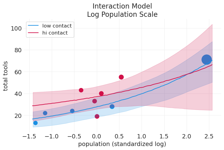
plot_tools_model_posterior_predictive(
    interaction_model,
    interaction_inference,
    title="Interaction Model\nLog Population Scale",
    plot_natural_scale=False,
)
Sampling: [tools]
Sampling: [tools]
plot_tools_model_posterior_predictive(
    interaction_model,
    interaction_inference,
    title="Interaction Model\nNatural Population Scale",
    plot_natural_scale=True,
)
Sampling: [tools]
Sampling: [tools]
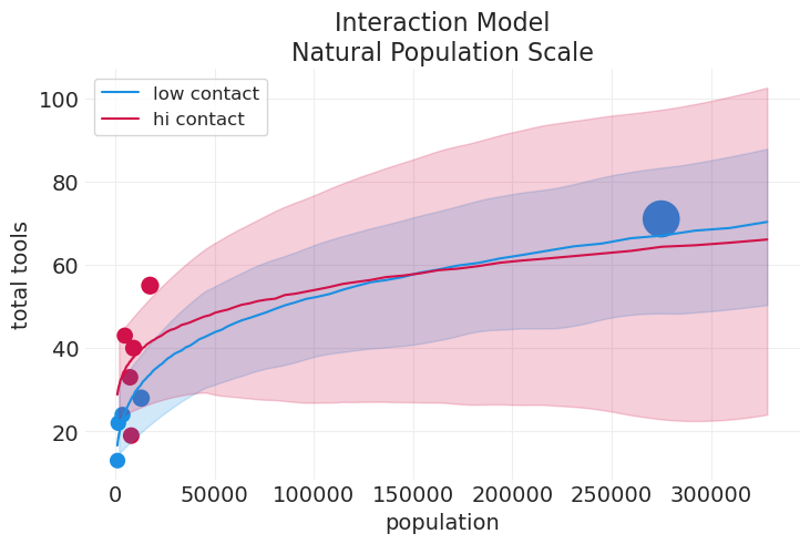
上面的模型之所以“糟糕”的原因如下:#
低接触均值与高接触均值相交(大约在 15 万人口左右)。这在逻辑上意义不大
人口 = 0 的截距应该非常接近 0。但对于两组而言,它都在 20 和 30 左右。
汤加甚至没有包含在高接触组的 89% HDI 中
对于大多数人口范围,高接触组的误差都非常大
我们能做得更好吗?
通过更好的科学模型改进估计器#
有两种立即改进模型的方法,包括
稳健回归模型 – 在这种情况下是伽玛-泊松(负二项式)模型
使用更符合原则的科学模型
包含创新和技术损失的科学模型#
回顾一下之前这个 DAG,它突出了关于观察到的工具如何产生的一般概念想法
utils.draw_causal_graph(
    edge_list=[
        ("Population", "Innovation"),
        ("Innovation", "Tools Developed"),
        ("Contact Level", "Innovation"),
        ("Tools Developed", "Tool Loss"),
        ("Tool Loss", "Total Tools Observed"),
    ],
    graph_direction="LR",
)
为什么不开发一个科学模型来做到这一点呢?
使用差分方程:\(\Delta T = \alpha P^\beta - \gamma T\)#
\(\Delta T\) 是在给定当前工具数量的情况下工具数量的变化。这里的 T 可以被认为是当前一代的工具数量
\(\alpha\) 是人口规模为 \(P\) 的创新率
\(\beta\) 是弹性,可以被认为是饱和率或“收益递减”因子;如果我们约束 \(0 > \beta < 1\)
\(\gamma\) 是时间 T 的损耗/技术损失率
此外,我们可以通过接触率等级 \(C\) 将这样的方程参数化为 \(\Delta T = \alpha_C P^{\beta_C} - \gamma T\)
现在我们利用均衡的概念来识别最终获得的稳态工具数量。此时 \(\Delta T = 0\),我们可以使用代数求解得到的 \(\hat T\)
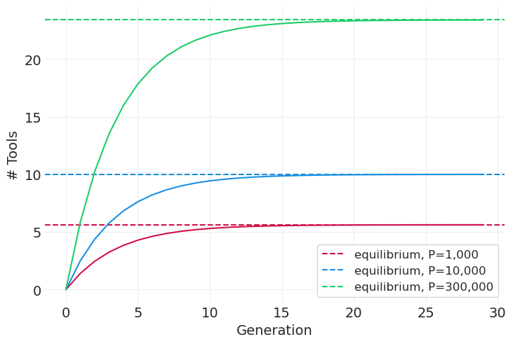
模拟不同社会的差分方程#
def simulate_tools(alpha=0.25, beta=0.25, P=1e3, gamma=0.25, n_generations=30, color="C0"):
    """Simulate the Tools data as additive difference process equilibrium condition"""

    def difference_equation(t):
        return alpha * P**beta - gamma * t

    # Run the simulation
    tools = [0]
    generations = range(n_generations)
    for g in generations:
        t = tools[-1]
        tools.append(t + difference_equation(t))

    t_equilibrium = (alpha * P**beta) / gamma

    # Plot it
    plt.plot(generations, tools[:-1], color=color)
    plt.axhline(t_equilibrium, color=color, linestyle="--", label=f"equilibrium, P={int(P):,}")
    plt.legend()


simulate_tools(P=1e3, color="C0")
simulate_tools(P=1e4, color="C1")
simulate_tools(P=300_000, color="C2")
plt.xlabel("Generation")
plt.ylabel("# Tools");
创新/损失统计模型#
使用 \(\hat T = \lambda\) 作为预期工具数量,即 \(T \sim \text{Poisson}(\hat T)\)
注意:我们必须约束 \(\lambda\) 为正数,我们可以通过几种方式做到这一点
对变量取指数
使用适当的先验来约束变量为正数(我们将使用这种方法)
确定良好的先验超参数#
我们将使用指数分布作为差分方程参数 \(\alpha, \beta, \gamma\) 的先验。因此,我们需要确定涵盖 0.25 = 1/4 的良好比率超参数 \(\eta\) 以用于这些先验。
所有参数的合理值在上面的模拟中约为 0.25。因此,我们希望确定涵盖 0.25 = 1/4 的指数率参数。
ETA = 4
with pm.Model(coords={"contact": CONTACT}) as innovation_loss_model:

    # Note: raw population here, not log/standardized
    population = pm.Data("population", POPULATION, dims="obs_id")
    contact_level = pm.Data("contact_level", CONTACT_LEVEL, dims="obs_id")

    # Priors -- we use Exponential for all.
    # Note that in the lecture: McElreath uses a Normal for alpha
    # then applies a exp(alpha) to enforce positive contact-level
    # innovation rate
    alpha = pm.Exponential("alpha", ETA, dims="contact")

    # contact-level elasticity
    beta = pm.Exponential("beta", ETA, dims="contact")

    # global technology loss rate
    gamma = pm.Exponential("gamma", ETA)

    # Likelihood using difference equation equilibrium as mean Poisson rate
    T_hat = (alpha[contact_level] * (population ** beta[contact_level])) / gamma
    pm.Poisson("tools", T_hat, observed=TOOLS, dims="obs_id")

    innovation_loss_inference = pm.sample(tune=2000, target_accept=0.98)
    # NOTE: For compute_log_likelihood to work for models that contain variables
    # with dims but no coords (e.g. dims="obs_ids"), we need the
    # following PR to be merged https://github.com/pymc-devs/pymc/pull/6882
    # (I've implemented the fix locally in pymc/stats/log_likelihood.py to
    # get analysis to execute)
    #
    # TODO: Once merged, update pymc version in conda environment
    innovation_loss_inference = pm.compute_log_likelihood(innovation_loss_inference)


pm.model_to_graphviz(innovation_loss_model)
Initializing NUTS using jitter+adapt_diag...
Multiprocess sampling (4 chains in 4 jobs)
NUTS: [alpha, beta, gamma]
Sampling 4 chains for 2_000 tune and 1_000 draw iterations (8_000 + 4_000 draws total) took 12 seconds.

az.summary(innovation_loss_inference)
| 均值 | 标准差 | hdi_3% | hdi_97% | mcse_mean | mcse_sd | ess_bulk | ess_tail | r_hat | |
|---|---|---|---|---|---|---|---|---|---|
| alpha[low] | 0.301 | 0.211 | 0.033 | 0.692 | 0.005 | 0.004 | 1249.0 | 1304.0 | 1.0 |
| alpha[high] | 0.314 | 0.246 | 0.011 | 0.752 | 0.006 | 0.004 | 1736.0 | 1762.0 | 1.0 |
| beta[low] | 0.261 | 0.034 | 0.197 | 0.325 | 0.001 | 0.001 | 1960.0 | 1710.0 | 1.0 |
| beta[high] | 0.296 | 0.105 | 0.100 | 0.493 | 0.003 | 0.002 | 1254.0 | 1039.0 | 1.0 |
| gamma | 0.115 | 0.085 | 0.007 | 0.270 | 0.002 | 0.002 | 1222.0 | 1278.0 | 1.0 |
我们可以看到,对于 \(\alpha\) 和 \(\beta\) 参数,最佳值在 0.23-0.28 左右。对于 gamma,它略小,约为 0.09。我们可以潜在地重新参数化我们的模型,使 Gamma 变量具有更紧密的先验,但算了。
后验预测#
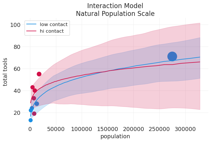
#### Replot the contact model for comparison
plot_tools_model_posterior_predictive(
    interaction_model,
    interaction_inference,
    title="Interaction Model\nNatural Population Scale",
    plot_natural_scale=True,
)
Sampling: [tools]
Sampling: [tools]
plot_tools_model_posterior_predictive(
    innovation_loss_model,
    innovation_loss_inference,
    title="Innovation Model\nNatural Population Scale",
    input_natural_scale=True,
    plot_natural_scale=True,
)
Sampling: [tools]
Sampling: [tools]
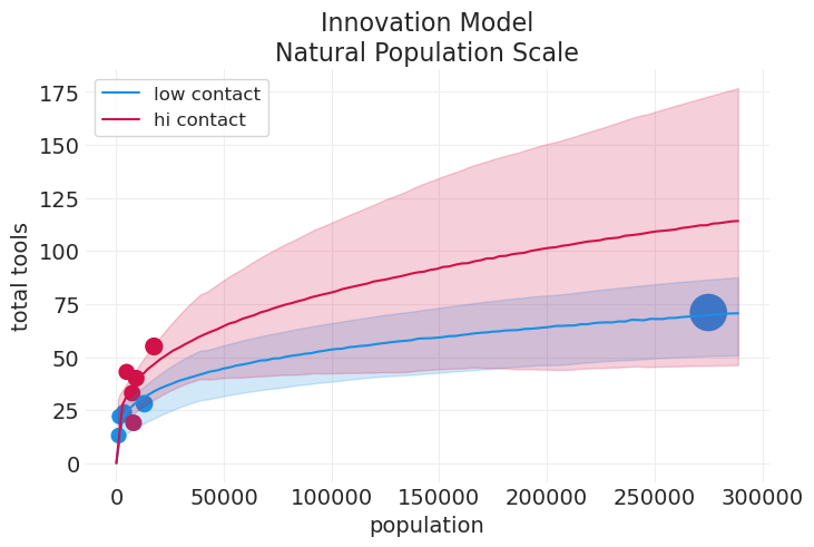
请注意基本交互模型之上的以下改进
低/高接触趋势没有奇怪的交叉
零人口现在与零工具相关联
模型比较#
compare_dict = {
    "global intercept": global_intercept_inference,
    "contact": interaction_inference,
    "innovation loss": innovation_loss_inference,
}
az.compare(compare_dict)
| 排名 | elpd_loo | p_loo | elpd_diff | 权重 | 标准误差 | dse | 警告 | 比例 | |
|---|---|---|---|---|---|---|---|---|---|
| 创新损失 | 0 | -40.892427 | 5.706997 | 0.000000 | 0.862233 | 5.666719 | 0.000000 | True | 对数 |
| 接触 | 1 | -42.799083 | 7.239629 | 1.906656 | 0.000000 | 6.275191 | 2.736439 | True | 对数 |
| 全局截距 | 2 | -71.152042 | 8.674912 | 30.259615 | 0.137767 | 16.274744 | 16.728641 | True | 对数 |
我们还可以看到,就 LOO 预测而言,创新/损失模型远优于(权重 = 0.94)。
要点#
通常最好有一个领域知情的科学模型
我们仍然有未观察到的位置混淆因素需要处理
回顾:计数 GLM#
MaxEnt 先验
二项分布
泊松分布及扩展
log链接函数;exp逆链接函数
稳健回归
Beta-二项分布
Gamma-泊松分布
奖励:辛普森的潘多拉魔盒#
当组被组合或分离时,某些测量/估计的关联的反转。
辛普森悖论没有什么特别有趣或悖论的地方
它只是一种统计现象
有许多因果现象可以产生 SP
管道和分叉会导致一种 SP – 即分层破坏趋势/关联
对撞机可能导致相反的 SP – 即分层引发趋势/关联
如果不做出明确的因果声明,你就无法说哪种“反转”方向是正确的
经典示例是加州大学伯克利分校的录取#
如果你不按院系分层/调节,你会发现女性的录取率较低
如果你按院系分层/调节,你会发现女性的录取率略高(参见上面的录取分析)
哪个是正确的?两者都可以解释
中介/管道(院系)
对撞机 + 混淆因素(未观察到的能力)
**有关管道、分叉和对撞机如何“导致”辛普森悖论的示例,请参见 讲座 05 – 基本混淆因素 **
非线性困扰#
虽然 \(Z\) 不是混淆因素,但它是 \(Y\) 的竞争原因。如果因果模型是非线性的,并且我们按 \(Z\) 分层以获得治疗对结果的直接因果效应,这可能会导致一些类似于辛普森悖论的奇怪结果。
utils.draw_causal_graph(edge_list=[("treatment, X", "outcome, Y"), ("covariate, Z", "outcome, Y")])

示例:基准率差异#
在这里,我们模拟数据,其中 \(X\) 和 \(Z\) 是独立的,但 \(Z\) 对 \(Y\) 具有非线性因果效应
生成模拟#
np.random.seed(123)
n_simulations = 1000
X = stats.norm.rvs(size=n_simulations)
Z = stats.bernoulli.rvs(p=0.5, size=n_simulations)
# encode a nonlinear effect of Z on Y
BETA_XY = 1
BETA_Z0Y = 5
BETA_Z1Y = -1
p = utils.invlogit(X * BETA_XY + np.where(Z, BETA_Z1Y, BETA_Z0Y))
Y = stats.bernoulli.rvs(p=p)
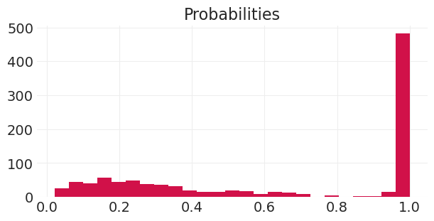
plt.subplots(figsize=(6, 3))
plt.hist(p, bins=25)
plt.title("Probabilities");
未分层模型 – \(\text{logit}(p_i) = \alpha + \beta X_i\)#
# Unstratified model
with pm.Model() as unstratified_model:

    # Data for PPDs
    x = pm.Data("X", X)

    # Global params
    alpha = pm.Normal("alpha", 0, 1)
    beta = pm.Normal("beta", 0, 1)

    # record p for plotting predictions
    p = pm.Deterministic("p", pm.math.invlogit(alpha + beta * x))
    pm.Bernoulli("Y", p=p, observed=Y)

    unstratified_inference = pm.sample()

pm.model_to_graphviz(unstratified_model)
Initializing NUTS using jitter+adapt_diag...
Multiprocess sampling (4 chains in 4 jobs)
NUTS: [alpha, beta]
Sampling 4 chains for 1_000 tune and 1_000 draw iterations (4_000 + 4_000 draws total) took 1 seconds.

部分分层模型 – \(\text{logit}(p) = \alpha + \beta_{Z[i]} X_i\)#
# Partially statified Model
with pm.Model() as partially_stratified_model:

    # Mutable data for PPDs
    x = pm.Data("X", X)
    z = pm.Data("Z", Z)

    alpha = pm.Normal("alpha", 0, 1)
    beta = pm.Normal("beta", 0, 1, shape=2)

    # record p for plotting predictions
    p = pm.Deterministic("p", pm.math.invlogit(alpha + beta[z] * x))
    pm.Bernoulli("Y", p=p, observed=Y)

    partially_stratified_inference = pm.sample()


pm.model_to_graphviz(partially_stratified_model)
Initializing NUTS using jitter+adapt_diag...
Multiprocess sampling (4 chains in 4 jobs)
NUTS: [alpha, beta]
Sampling 4 chains for 1_000 tune and 1_000 draw iterations (4_000 + 4_000 draws total) took 1 seconds.

未分层模型后验预测#
# Get predictions -- unstratified model
RESOLUTION = 100
xs = np.linspace(-3, 3, RESOLUTION)

with unstratified_model:
    pm.set_data({"X": xs})
    unstratified_ppd = pm.sample_posterior_predictive(unstratified_inference, var_names=["p"])[
        "posterior_predictive"
    ]["p"]
Sampling: []
部分分层模型后验预测#
# Get predictions -- partially stratified model
partially_stratified_predictions = {}
with partially_stratified_model:
    for z in [0, 1]:
        # Z = 0 predictions
        pm.set_data({"X": xs})
        pm.set_data({"Z": [z] * RESOLUTION})
        partially_stratified_predictions[z] = pm.sample_posterior_predictive(
            partially_stratified_inference, var_names=["p"]
        )["posterior_predictive"]["p"]
Sampling: []
Sampling: []
绘制分层效果图#
from matplotlib.lines import Line2D

n_posterior_samples = 20
_, axs = plt.subplots(1, 2, figsize=(8, 4))
plt.sca(axs[0])

# Plot predictions -- unstratified model
plt.plot(xs, unstratified_ppd.sel(chain=0)[:n_posterior_samples].T, color="C0")
plt.xlabel("treatment, X")
plt.ylabel("p(Y)")
plt.ylim([0, 1])
plt.title("$logit(p_i) = \\alpha + \\beta x_i$")

# For tagging conditions in legend
legend_data = [
    Line2D([0], [0], color="C0", lw=4),
    Line2D([0], [0], color="C1", lw=4),
]


plt.sca(axs[1])
for z in [0, 1]:
    ys = partially_stratified_predictions[z].sel(chain=0)[:n_posterior_samples].T
    plt.plot(xs, ys, color=f"C{z}", label=f"Z={z}")

plt.xlabel("treatment, X")
plt.ylabel("p(Y)")
plt.ylim([0, 1])

plt.legend(legend_data, ["Z=0", "Z=1"])

plt.title("$logit(p_i) = \\alpha + \\beta_{Z[i]}x_i$")

plt.sca(axs[0])
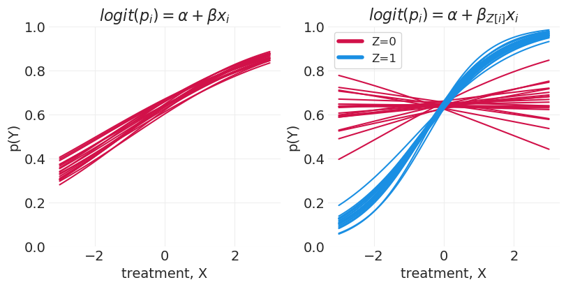
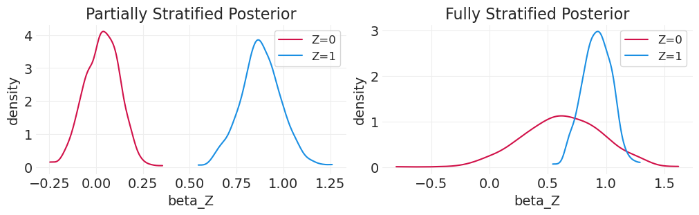
当仅对 X 系数进行分层,从而共享一个共同的截距时,我们可以看到对于 Z=0,在 0.6 左右存在饱和。这是由于在逻辑回归模型中,Y|Z=0 的对数几率增加了 +5。由于这种饱和,很难判断治疗是否对该组的结果产生影响。
_, axs = plt.subplots(figsize=(5, 3))
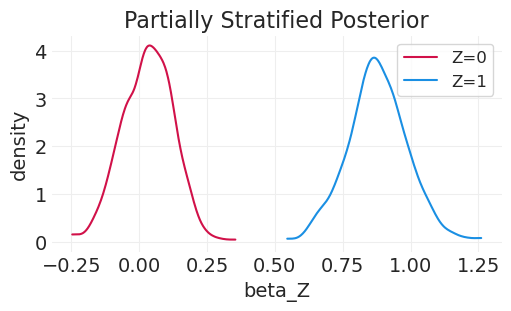
for z in [0, 1]:
post = partially_stratified_inference.posterior.sel(chain=0)["beta"][:, z]
az.plot_dist(post, color=f"C{z}", label=f"Z={z}")
plt.xlabel("beta_Z")
plt.ylabel("density")
plt.legend()
plt.title("Partially Stratified Posterior");
尝试完全分层模型 – \(\text{logit}(p_i) = \alpha_{Z[i]} + \beta_{Z[i]}X_i\)#
为每个组包含单独的截距
# Fully statified Model
with pm.Model() as fully_stratified_model:

    x = pm.Data("X", X)
    z = pm.Data("Z", Z)

    # Stratify intercept by Z as well
    alpha = pm.Normal("alpha", 0, 1, shape=2)
    beta = pm.Normal("beta", 0, 1, shape=2)

    # Log p for plotting predictions
    p = pm.Deterministic("p", pm.math.invlogit(alpha[z] + beta[z] * x))
    pm.Bernoulli("Y", p=p, observed=Y)
    fully_stratified_inference = pm.sample()


pm.model_to_graphviz(fully_stratified_model)
Initializing NUTS using jitter+adapt_diag...
Multiprocess sampling (4 chains in 4 jobs)
NUTS: [alpha, beta]
Sampling 4 chains for 1_000 tune and 1_000 draw iterations (4_000 + 4_000 draws total) took 1 seconds.

完全分层模型后验预测#
# Get predictions -- partially stratified model
fully_stratified_predictions = {}
with fully_stratified_model:
    for z in [0, 1]:
        # Z = 0 predictions
        pm.set_data({"X": xs})
        pm.set_data({"Z": [z] * RESOLUTION})
        fully_stratified_predictions[z] = pm.sample_posterior_predictive(
            fully_stratified_inference, var_names=["p"]
        )["posterior_predictive"]["p"]
Sampling: []
Sampling: []
n_posterior_samples = 20
_, axs = plt.subplots(1, 2, figsize=(8, 4))
plt.sca(axs[0])

for z in [0, 1]:
    ys = partially_stratified_predictions[z].sel(chain=0)[:n_posterior_samples].T
    plt.plot(xs, ys, color=f"C{z}", label=f"Z={z}")

plt.xlabel("treatment, X")
plt.ylabel("p(Y)")
plt.ylim([0, 1])

plt.legend(legend_data, ["Z=0", "Z=1"])
plt.title("$logit(p_i) = \\alpha + \\beta_{Z[i]}X_i$")

plt.sca(axs[1])
for z in [0, 1]:
    ys = fully_stratified_predictions[z].sel(chain=0)[:n_posterior_samples].T
    plt.plot(xs, ys, color=f"C{z}", label=f"Z={z}")

plt.xlabel("Treatment, X")
plt.ylabel("p(Y)")
plt.ylim([0, 1])

plt.legend(legend_data, ["Z=0", "Z=1"])

plt.title("$logit(p_i) = \\alpha_{Z[i]} + \\beta_{Z[i]}X_i$");
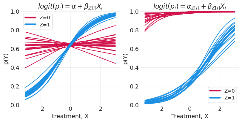
在这里,我们可以看到,使用完全分层模型(其中我们包含组级截距),Z=0 的预测甚至更高地向上移动到 1,尽管对于治疗 X 的所有值,预测仍然基本持平
比较后验分布#
_, axs = plt.subplots(1, 2, figsize=(10, 3))

plt.sca(axs[0])

for z in [0, 1]:
    post = partially_stratified_inference.posterior.sel(chain=0)["beta"][:, z]
    az.plot_dist(post, color=f"C{z}", label=f"Z={z}")
plt.xlabel("beta_Z")
plt.ylabel("density")
plt.legend()
plt.title("Partially Stratified Posterior")


plt.sca(axs[1])
for z in [0, 1]:
    post = fully_stratified_inference.posterior.sel(chain=0)["beta"][:, z]
    az.plot_dist(post, color=f"C{z}", label=f"Z={z}")
plt.xlabel("beta_Z")
plt.ylabel("density")
plt.legend()
plt.title("Fully Stratified Posterior");
辛普森悖论总结#
没有悖论,几乎任何事物都可能产生辛普森悖论 (SP)
系数反转在因果框架之外几乎没有解释价值
不要关注系数:通过模型推送预测以进行比较
随机提示:你不能接受零假设,你只能拒绝它。
仅仅因为分布与 0 重叠并不意味着它为零
许可声明#
本示例库中的所有笔记本均根据 MIT 许可证 提供,该许可证允许修改和再分发以用于任何用途,前提是保留版权和许可声明。
引用 PyMC 示例#
要引用此笔记本,请使用 Zenodo 为 pymc-examples 仓库提供的 DOI。
重要提示
许多笔记本改编自其他来源:博客、书籍……在这种情况下,您也应该引用原始来源。
另请记住引用您的代码使用的相关库。
这是一个 bibtex 中的引用模板
@incollection{citekey,
  author    = "<notebook authors, see above>",
  title     = "<notebook title>",
  editor    = "PyMC Team",
  booktitle = "PyMC examples",
  doi       = "10.5281/zenodo.5654871"
}
渲染后可能如下所示