


有序类别#
本笔记本是 PyMC 端口的一部分,该端口移植自 Richard McElreath 的 Statistical Rethinking 2023 系列讲座。
视频 - 第 11 讲 - 有序类别# 第 11 讲 - 有序类别
# Ignore warnings
import warnings

import arviz as az
import numpy as np
import pandas as pd
import pymc as pm
import statsmodels.formula.api as smf
import utils as utils
import xarray as xr

from matplotlib import pyplot as plt
from matplotlib import style
from scipy import stats as stats

warnings.filterwarnings("ignore")

# Set matplotlib style
STYLE = "statistical-rethinking-2023.mplstyle"
style.use(STYLE)
解决科学问题#
当解决知识边缘的问题时#
通常没有可用的算法来告诉你如何解决它
我们能做的最好的就是看大量的例子
推导出一套通用的启发式方法来解决问题
尝试解决一个更易于访问的问题或子问题
例如,先尝试构建一个更简单的模型,然后再增加复杂性
始终检查你的工作 - 例如,通过模拟
你并不总是得到你想要的#
可能无法估计所需的估计量
你可能不得不妥协
例如,估计总效应与直接效应
敏感性分析
估计反事实
伦理与电车难题研究#
研究原则#
研究人员试图沿着多个特征维度对电车难题场景进行分类,三个常见的特征是
行动:采取行动在道德上不如不采取行动那么被允许(你干预一个场景被认为比让场景自行发展更糟糕)
意图:行为者的直接目标是否影响场景(例如,故意杀死一个人以拯救五个人)
接触:如果行为者与行动对象直接接触,则意图更糟糕(例如,直接将一个人从桥上推下以拯救他人)
数据集#
TROLLEY = utils.load_data("Trolley")
N_TROLLEY_RESPONSES = len(TROLLEY)
N_RESPONSE_CATEGORIES = TROLLEY.response.max()
TROLLEY.head()
| 案例 | 响应 | 顺序 | ID | 年龄 | 男性 | 教育程度 | 行动 | 意图 | 接触 | 故事 | 行动2 | |
|---|---|---|---|---|---|---|---|---|---|---|---|---|
| 0 | cfaqu | 4 | 2 | 96;434 | 14 | 0 | 中学 | 0 | 0 | 1 | aqu | 1 |
| 1 | cfbur | 3 | 31 | 96;434 | 14 | 0 | 中学 | 0 | 0 | 1 | bur | 1 |
| 2 | cfrub | 4 | 16 | 96;434 | 14 | 0 | 中学 | 0 | 0 | 1 | rub | 1 |
| 3 | cibox | 3 | 32 | 96;434 | 14 | 0 | 中学 | 0 | 1 | 1 | box | 1 |
| 4 | cibur | 3 | 4 | 96;434 | 14 | 0 | 中学 | 0 | 1 | 1 | bur | 1 |
总共 9330 个响应
331 位个体
30 种不同的电车难题场景
沿行动、意图、接触维度变化
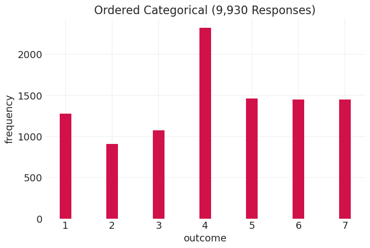
响应是从 1 到 7 的有序整数值,表示行动的“适当性”
不是计数
有序但不是连续有序
有界
response_counts = TROLLEY.groupby("response").count()["action"]
bars = plt.bar(response_counts.index, response_counts.values, width=0.25)
plt.xlabel("outcome")
plt.ylabel("frequency")
plt.title(f"Ordered Categorical ({N_TROLLEY_RESPONSES:,} Responses)");
估计量 行动、意图和接触 如何影响 响应
utils.draw_causal_graph(
    edge_list=[("X", "R"), ("S", "R"), ("E", "R"), ("Y", "R"), ("G", "R"), ("Y", "E"), ("G", "E")],
    node_props={
        "X": {"color": "blue", "label": "action, intenition, contact, X"},
        "R": {"color": "red", "label": "response, R"},
        "S": {"label": "story, S"},
        "E": {"label": "education, E"},
        "Y": {"label": "age, Y"},
        "G": {"label": "gender, G"},
    },
    edge_props={
        ("X", "R"): {"color": "red"},
    },
    graph_direction="LR",
)

有序类别#
离散类别
类别具有顺序,因此 7 > 6 > 5,等等,但 7 不一定比 1 大 7 倍
每个值之间的距离不是恒定的,也不清楚
锚点(例如,这里的 4 是“一般般”)
不同的人有不同的锚点
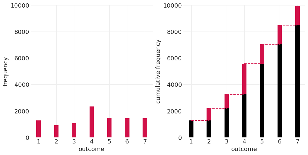
有序 = 累积#
而不是 \(p(x=5)\), \(p(x<=5)\)
累积分布函数#
fig, axs = plt.subplots(1, 2, figsize=(10, 5))
xticks = range(1, 8)

cumulative_counts = response_counts.cumsum()

plt.sca(axs[0])
plt.bar(response_counts.index, response_counts.values, color="C0", width=0.25)
plt.xlabel("outcome")
plt.xticks(xticks)
plt.ylabel("frequency")
plt.ylim([0, 10_000])

# Cumulative frequency
plt.sca(axs[1])
plt.bar(response_counts.index, cumulative_counts.values, color="k", width=0.25)
offsets = cumulative_counts.values[1:] - response_counts.values[1:]
plt.bar(
    cumulative_counts.index[1:], response_counts.values[1:], bottom=offsets, color="C0", width=0.25
)

for ii, y in enumerate(offsets):
    x0 = ii + 1
    x1 = x0 + 1
    plt.plot((x0, x1), (y, y), color="C0", linestyle="--")

plt.xlabel("outcome")
plt.xticks(xticks)
plt.ylabel("cumulative frequency")
plt.ylim([0, 10_000]);
累积对数优势比#
fig, axs = plt.subplots(1, 2, figsize=(10, 5))

response_probs = response_counts / response_counts.sum()
cumulative_probs = response_probs.cumsum()

# Plot  Cumulative proportion
plt.sca(axs[0])
plt.bar(cumulative_probs.index, cumulative_probs.values, color="k", width=0.25)
offsets = cumulative_probs.values - response_probs.values
plt.bar(cumulative_probs.index, response_probs.values, bottom=offsets, color="C0", width=0.25)

offsets = np.append(offsets, 1)  # add p = 1 condition
for ii, y in enumerate(offsets[1:]):
    x1 = ii + 1
    plt.plot((0, x1), (y, y), color="C0", linestyle="--")

plt.xlabel("outcome")
plt.xticks(xticks)
plt.xlim([0, 7.5])
plt.ylabel("cumulative proportion")
plt.ylim([0, 1.05])

# Cumulative proportion vs cumulative log-odds
infty = 3.5  # "Infinity" log odds x-value for plots
neg_infty = -1 * infty
cumulative_log_odds = [np.log(p / (1 - p)) for p in cumulative_probs]
cumulative_log_odds[-1] = infty

# Plot cumulative data points
plt.sca(axs[1])
plt.scatter(cumulative_log_odds, cumulative_probs.values, color="C1", s=100)
plt.scatter(infty, 1, color="gray", s=100)  # add point for Infinity
for ii, (clo, clp) in enumerate(zip(cumulative_log_odds, cumulative_probs.values)):

    # Add cumulative proportion
    plt.plot((neg_infty, clo), (clp, clp), color="C0", linestyle="--")

    # Add & label cutpoints
    if ii < N_RESPONSE_CATEGORIES - 1:
        plt.plot((clo, clo), (0, clp), color="C1", linestyle="--")
        plt.text(clo + 0.05, 0.025, f"$\\alpha_{ii+1}$", color="C1", fontsize=10)
    else:
        plt.plot((clo, clo), (0, clp), color="grey", linestyle="--")

    # Annotate data points
    plt.text(clo + 0.05, clp + 0.02, f"{ii+1}", color="C1", fontsize=20)

plt.xlabel("cumulative log-odds")
plt.xlim([neg_infty, infty + 0.5])
plt.xticks([-2, 0, 2, infty], labels=[-2, 0, 2, "$\\infty$"])
plt.ylabel("cumulative proportion")
plt.ylim([0, 1.05])

plt.sca(axs[0])
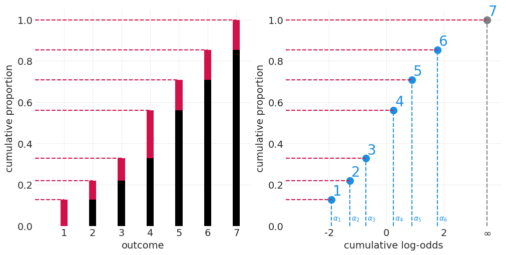
使用 CDF 对响应进行排序#
使用 CDF,我们可以在累积对数优势比上建立切割点 \(\alpha_R\),这些切割点与该响应(或更小的响应)的累积概率相对应。因此,CDF 为我们提供了顺序的代理。
计算 \(P(R_i=k)\)#
例如,对于 \(k = 3\)
设置 GLM#
我们将累积对数优势比建模为每个断点 \(\alpha_k\)
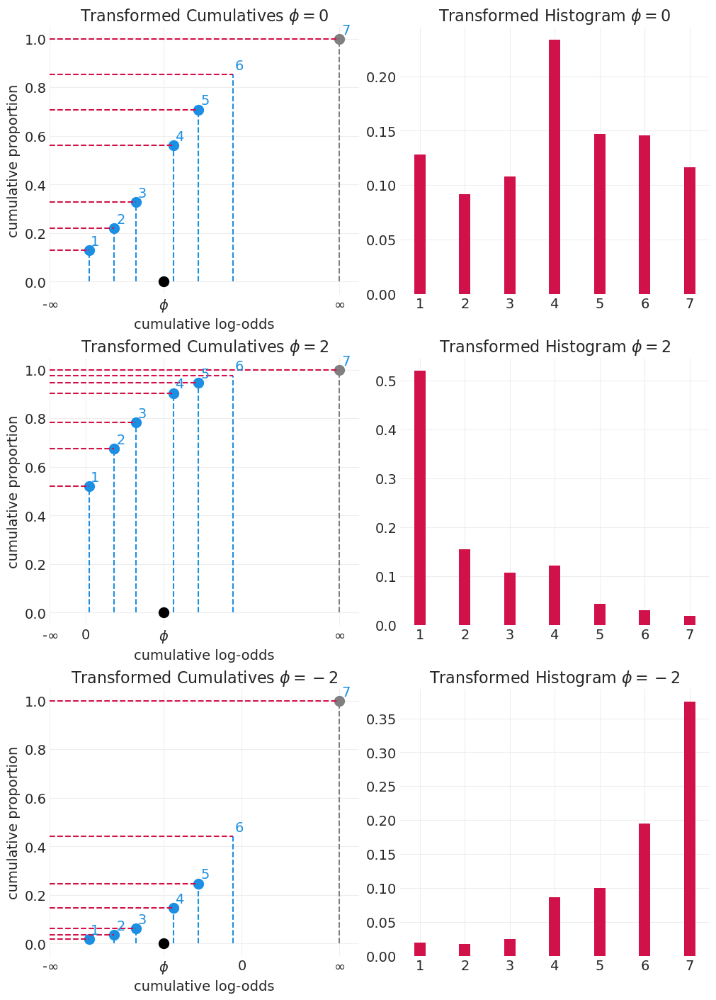
GLM 在哪里?#
我们如何使它成为预测变量的函数
为每个预测变量设置一个 \(\alpha_k\)
为每个数据点使用偏移量 \(\phi_i\),该偏移量是预测变量的函数
演示 \(\phi\) 对响应分布的影响#
更改 \(\phi\) 会“挤压”或“拉伸”累积直方图
def plot_cumulative_log_odds_and_cumulative_probs(cumulative_log_odds, cumulative_probs, phi):
    infity = max(cumulative_log_odds) + 1
    neg_infity = min(cumulative_log_odds) - 1

    # Plot cumulative data points
    plt.scatter(cumulative_log_odds[:-2], cumulative_probs[:-2], color="C1", s=100)
    plt.scatter(infity, 1, color="gray", s=100)  # add point for Infinity

    for ii, (clo, clp) in enumerate(zip(cumulative_log_odds, cumulative_probs)):

        # Add & label cutpoints
        if ii < N_RESPONSE_CATEGORIES - 1:
            plt.plot((clo, clo), (0, clp), color="C1", linestyle="--")
            # Add cumulative proportion
            plt.plot((neg_infity, clo), (clp, clp), color="C0", linestyle="--")
            # Annotate data points
            plt.text(clo + 0.05, clp + 0.02, f"{ii+1}", color="C1", fontsize=14)
        else:
            plt.plot((infity, infity), (0, 1), color="grey", linestyle="--")
            plt.plot((neg_infity, infity), (1, 1), color="C0", linestyle="--")
            # Annotate data points
            plt.text(infity + 0.05, 1 + 0.02, f"{ii+1}", color="C1", fontsize=14)

    plt.xlabel("cumulative log-odds")
    plt.xlim([neg_infity, infity + 0.5])
    if phi < 0:
        xticks = [neg_infity, phi, 0, infity]
        xtick_labels = ["-$\\infty$", "$\\phi$", 0, "$\\infty$"]
    elif phi > 0:
        xticks = [neg_infity, 0, phi, infity]
        xtick_labels = ["-$\\infty$", 0, "$\\phi$", "$\\infty$"]
    else:
        xticks = [neg_infity, phi, infity]
        xtick_labels = ["-$\\infty$", "$\\phi$", "$\\infty$"]

    plt.xticks(xticks, labels=xtick_labels)
    plt.ylabel("cumulative proportion")
    plt.ylim([-0.05, 1.05])


def plot_cumulative_probs_bar(cumulative_probs):
    xs = range(1, len(cumulative_probs) + 1)
    diff_probs = [c for c in cumulative_probs]
    diff_probs.insert(0, 0)
    probs = np.diff(diff_probs)
    plt.bar(xs, probs, color="C0", width=0.25)


def show_phi_effect(cumulative_log_odds, phi=0):
    if not isinstance(phi, list):
        phi = [phi]
    n_phis = len(phi)

    fig, axs = plt.subplots(n_phis, 2, figsize=(10, 8 + n_phis * 2))

    for ii, ph in enumerate(phi):

        # Shift the cumulative log odds by phi
        cumulative_log_odds_plus_phi = [v + ph for v in cumulative_log_odds]

        # Resulting cumulative probabilities
        cumulative_probs_plus_phi = [utils.invlogit(c) for c in cumulative_log_odds_plus_phi]

        plt.sca(axs[ii][0])

        plot_cumulative_log_odds_and_cumulative_probs(
            cumulative_log_odds=cumulative_log_odds_plus_phi,
            cumulative_probs=cumulative_probs_plus_phi,
            phi=ph,
        )
        plt.scatter(ph, 0, s=100, color="k")
        plt.title(f"Transformed Cumulatives $\\phi={ph}$")

        plt.sca(axs[ii][1])
        plot_cumulative_probs_bar(cumulative_probs_plus_phi)
        plt.title(f"Transformed Histogram $\\phi={ph}$")


show_phi_effect(cumulative_log_odds, phi=[0, 2, -2])
统计模型#
从简单的开始#
utils.draw_causal_graph(
    edge_list=[("X", "R"), ("S", "R"), ("E", "R"), ("Y", "R"), ("G", "R"), ("Y", "E"), ("G", "E")],
    node_props={
        "X": {"color": "red", "label": "action, intenition, contact, X"},
        "R": {"color": "red", "label": "response, R"},
        "S": {"label": "story, S"},
        "E": {"label": "education, E"},
        "Y": {"label": "age, Y"},
        "G": {"label": "gender, G"},
    },
    edge_props={
        ("X", "R"): {"color": "red"},
    },
    graph_direction="LR",
)

# Set up data / coords
RESPONSE_ID, RESPONSE = pd.factorize(TROLLEY.response.astype(int), sort=True)
N_RESPONSE_CLASSES = len(RESPONSE)
CUTPOINTS = np.arange(1, N_RESPONSE_CLASSES).astype(int)

# for labeling cutpoints
coords = {"CUTPOINTS": CUTPOINTS}
with pm.Model(coords=coords) as basic_ordered_logistic_model:

    # Data for posetior predictions
    action = pm.Data("action", TROLLEY.action.astype(float))
    intent = pm.Data("intent", TROLLEY.intention.astype(float))
    contact = pm.Data("contact", TROLLEY.contact.astype(float))

    # Priors
    beta_action = pm.Normal("beta_action", 0, 0.5)
    beta_intent = pm.Normal("beta_intent", 0, 0.5)
    beta_contact = pm.Normal("beta_contact", 0, 0.5)

    cutpoints = pm.Normal(
        "alpha",
        mu=0,
        sigma=1,
        transform=pm.distributions.transforms.univariate_ordered,
        shape=N_RESPONSE_CLASSES - 1,
        initval=np.arange(N_RESPONSE_CLASSES - 1)
        - 2.5,  # use ordering (with coarse log-odds centering) for init
        dims="CUTPOINTS",
    )

    # Likelihood
    phi = beta_action * action + beta_intent * intent + beta_contact * contact
    pm.OrderedLogistic("response", cutpoints=cutpoints, eta=phi, observed=RESPONSE_ID)

pm.model_to_graphviz(basic_ordered_logistic_model)

with basic_ordered_logistic_model:
    basic_ordered_logistic_inference = pm.sample()
Initializing NUTS using jitter+adapt_diag...
Multiprocess sampling (4 chains in 4 jobs)
NUTS: [beta_action, beta_intent, beta_contact, alpha]
Sampling 4 chains for 1_000 tune and 1_000 draw iterations (4_000 + 4_000 draws total) took 38 seconds.
az.summary(
    basic_ordered_logistic_inference,
    var_names=["beta_contact", "beta_intent", "beta_action", "alpha"],
)
| 平均值 | 标准差 | hdi_3% | hdi_97% | mcse_mean | mcse_sd | ess_bulk | ess_tail | r_hat | |
|---|---|---|---|---|---|---|---|---|---|
| beta_contact | -0.943 | 0.050 | -1.032 | -0.849 | 0.001 | 0.001 | 3029.0 | 2894.0 | 1.0 |
| beta_intent | -0.711 | 0.036 | -0.777 | -0.644 | 0.001 | 0.000 | 3348.0 | 3184.0 | 1.0 |
| beta_action | -0.695 | 0.040 | -0.770 | -0.622 | 0.001 | 0.001 | 2522.0 | 3032.0 | 1.0 |
| alpha[1] | -2.819 | 0.046 | -2.898 | -2.726 | 0.001 | 0.001 | 1769.0 | 2416.0 | 1.0 |
| alpha[2] | -2.138 | 0.041 | -2.214 | -2.058 | 0.001 | 0.001 | 1919.0 | 2408.0 | 1.0 |
| alpha[3] | -1.556 | 0.039 | -1.625 | -1.479 | 0.001 | 0.001 | 2038.0 | 2547.0 | 1.0 |
| alpha[4] | -0.537 | 0.036 | -0.610 | -0.472 | 0.001 | 0.001 | 2402.0 | 3133.0 | 1.0 |
| alpha[5] | 0.131 | 0.037 | 0.066 | 0.204 | 0.001 | 0.001 | 2475.0 | 2695.0 | 1.0 |
| alpha[6] | 1.037 | 0.040 | 0.960 | 1.108 | 0.001 | 0.001 | 2825.0 | 3296.0 | 1.0 |
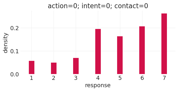
后验预测分布#
def run_basic_trolley_counterfactual(action=0, intent=0, contact=0, ax=None):
with basic_ordered_logistic_model:
pm.set_data(
{
"action": xr.DataArray([action] * N_TROLLEY_RESPONSES),
"intent": xr.DataArray([intent] * N_TROLLEY_RESPONSES),
"contact": xr.DataArray([contact] * N_TROLLEY_RESPONSES),
}
)
ppd = pm.sample_posterior_predictive(
basic_ordered_logistic_inference, extend_inferencedata=False
)
# recode back to 1-7
posterior_predictive = ppd.posterior_predictive["response"] + 1
# Posterior predictive density. Due to idiosyncracies with plt.hist(),
# az.plot_density() refuses to center on integer ticks, so we just do
# it manually with numpy and plt.bar()
if ax is not None:
plt.sca(ax)
else:
plt.subplots(figsize=(6, 3))
counts, bins = np.histogram(posterior_predictive.values.ravel(), bins=np.arange(1, 9))
total_counts = counts.sum()
counts = [c / total_counts for c in counts]
plt.bar(bins[:-1], counts, width=0.25)
plt.xlim([0.5, 7.5])
plt.xlabel("response")
plt.ylabel("density")
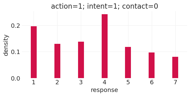
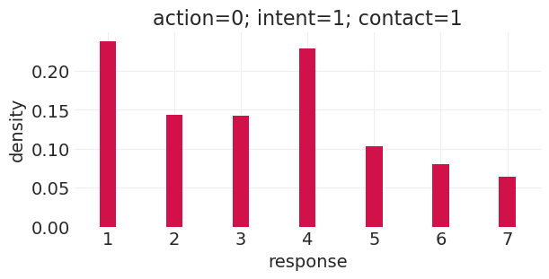
plt.title(f"action={action}; intent={intent}; contact={contact}")
run_basic_trolley_counterfactual(action=0, intent=0, contact=0)
Sampling: [response]
run_basic_trolley_counterfactual(action=1, intent=1, contact=0)
Sampling: [response]
run_basic_trolley_counterfactual(action=0, intent=1, contact=1)
Sampling: [response]
竞争原因呢?#
utils.draw_causal_graph(
    edge_list=[("X", "R"), ("S", "R"), ("E", "R"), ("Y", "R"), ("G", "R"), ("Y", "E"), ("G", "E")],
    node_props={
        "X": {"color": "red", "label": "action, intenition, contact, X"},
        "R": {"color": "red", "label": "response, R"},
        "S": {"label": "story, S"},
        "E": {"label": "education, E"},
        "Y": {"label": "age, Y"},
        "G": {"label": "gender, G"},
    },
    edge_props={
        ("X", "R"): {"color": "red"},
        ("Y", "R"): {"color": "blue"},
        ("E", "R"): {"color": "blue"},
        ("S", "R"): {"color": "blue"},
        ("G", "R"): {"color": "blue"},
    },
    graph_direction="LR",
)

性别的总效应#
utils.draw_causal_graph(
    edge_list=[("X", "R"), ("S", "R"), ("E", "R"), ("Y", "R"), ("G", "R"), ("Y", "E"), ("G", "E")],
    node_props={
        "X": {"label": "action, intenition, contact, X", "color": "red"},
        "R": {"color": "red", "label": "response, R"},
        "S": {"label": "story, S"},
        "E": {"label": "education, E"},
        "Y": {"label": "age, Y"},
        "G": {"label": "gender, G", "color": "blue"},
    },
    edge_props={
        ("G", "R"): {"color": "blue"},
        ("G", "E"): {"color": "blue"},
        ("E", "R"): {"color": "blue"},
        ("X", "R"): {"color": "red"},
    },
    graph_direction="LR",
)

拟合按性别分层的模型#
GENDER_ID, GENDER = pd.factorize(["M" if m else "F" for m in TROLLEY.male.values])

coords = {"GENDER": GENDER, "CUTPOINTS": CUTPOINTS}
with pm.Model(coords=coords) as total_effect_gender_model:

    # Data for posetior predictions
    action = pm.Data("action", TROLLEY.action.astype(float))
    intent = pm.Data("intent", TROLLEY.intention.astype(float))
    contact = pm.Data("contact", TROLLEY.contact.astype(float))
    gender = pm.Data("gender", GENDER_ID)

    # Priors
    beta_action = pm.Normal("beta_action", 0, 0.5, dims="GENDER")
    beta_intent = pm.Normal("beta_intent", 0, 0.5, dims="GENDER")
    beta_contact = pm.Normal("beta_contact", 0, 0.5, dims="GENDER")

    cutpoints = pm.Normal(
        "alpha",
        mu=0,
        sigma=1,
        transform=pm.distributions.transforms.univariate_ordered,
        shape=N_RESPONSE_CLASSES - 1,
        initval=np.arange(N_RESPONSE_CLASSES - 1)
        - 2.5,  # use ordering (with coarse log-odds centering) for init
        dims="CUTPOINTS",
    )

    # Likelihood
    phi = (
        beta_action[gender] * action + beta_intent[gender] * intent + beta_contact[gender] * contact
    )

    pm.OrderedLogistic("response", cutpoints=cutpoints, eta=phi, observed=RESPONSE_ID)

pm.model_to_graphviz(total_effect_gender_model)

with total_effect_gender_model:
    total_effect_gender_inference = pm.sample()
Initializing NUTS using jitter+adapt_diag...
Multiprocess sampling (4 chains in 4 jobs)
NUTS: [beta_action, beta_intent, beta_contact, alpha]
Sampling 4 chains for 1_000 tune and 1_000 draw iterations (4_000 + 4_000 draws total) took 41 seconds.
az.summary(
    total_effect_gender_inference, var_names=["beta_action", "beta_intent", "beta_contact", "alpha"]
)
| 平均值 | 标准差 | hdi_3% | hdi_97% | mcse_mean | mcse_sd | ess_bulk | ess_tail | r_hat | |
|---|---|---|---|---|---|---|---|---|---|
| beta_action[F] | -0.880 | 0.051 | -0.985 | -0.791 | 0.001 | 0.001 | 3392.0 | 2771.0 | 1.0 |
| beta_action[M] | -0.527 | 0.047 | -0.618 | -0.441 | 0.001 | 0.001 | 3353.0 | 3070.0 | 1.0 |
| beta_intent[F] | -0.895 | 0.048 | -0.981 | -0.802 | 0.001 | 0.001 | 3386.0 | 3078.0 | 1.0 |
| beta_intent[M] | -0.554 | 0.044 | -0.634 | -0.467 | 0.001 | 0.001 | 3778.0 | 2637.0 | 1.0 |
| beta_contact[F] | -1.059 | 0.066 | -1.181 | -0.935 | 0.001 | 0.001 | 3581.0 | 3001.0 | 1.0 |
| beta_contact[M] | -0.834 | 0.061 | -0.948 | -0.721 | 0.001 | 0.001 | 3350.0 | 2956.0 | 1.0 |
| alpha[1] | -2.828 | 0.046 | -2.913 | -2.740 | 0.001 | 0.001 | 2141.0 | 2476.0 | 1.0 |
| alpha[2] | -2.147 | 0.041 | -2.221 | -2.069 | 0.001 | 0.001 | 2068.0 | 2628.0 | 1.0 |
| alpha[3] | -1.562 | 0.038 | -1.631 | -1.489 | 0.001 | 0.001 | 2153.0 | 2425.0 | 1.0 |
| alpha[4] | -0.530 | 0.036 | -0.599 | -0.466 | 0.001 | 0.000 | 2609.0 | 2927.0 | 1.0 |
| alpha[5] | 0.145 | 0.035 | 0.077 | 0.207 | 0.001 | 0.000 | 2808.0 | 3497.0 | 1.0 |
| alpha[6] | 1.059 | 0.039 | 0.990 | 1.134 | 0.001 | 0.000 | 3410.0 | 3540.0 | 1.0 |
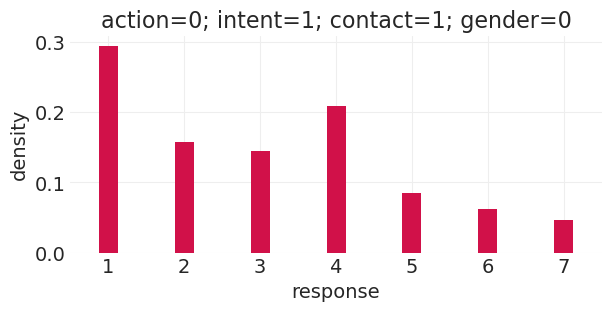
运行反事实#
def run_total_gender_counterfactual(action=0, intent=0, contact=0, gender=0, ax=None):
    with total_effect_gender_model:
        # hrmm, xr.DataArray doesn't seem to facilitate / speed up predictions 🤔
        pm.set_data(
            {
                "action": xr.DataArray([action] * N_TROLLEY_RESPONSES),
                "intent": xr.DataArray([intent] * N_TROLLEY_RESPONSES),
                "contact": xr.DataArray([contact] * N_TROLLEY_RESPONSES),
                "gender": xr.DataArray([gender] * N_TROLLEY_RESPONSES),
            }
        )
        ppd = pm.sample_posterior_predictive(
            total_effect_gender_inference, extend_inferencedata=False
        )

    # recode back to 1-7
    posterior_predictive = ppd.posterior_predictive["response"] + 1

    # Posterior predictive density. Due to idiosyncracies with plt.hist(),
    # az.plot_density() refuses to center on integer ticks, so we just do
    # it manually with numpy and plt.bar()
    if ax is not None:
        plt.sca(ax)
    else:
        plt.subplots(figsize=(6, 3))
    counts, bins = np.histogram(posterior_predictive.values.ravel(), bins=np.arange(1, 9))
    total_counts = counts.sum()
    counts = [c / total_counts for c in counts]
    plt.bar(bins[:-1], counts, width=0.25)

    plt.xlim([0.5, 7.5])
    plt.xlabel("response")
    plt.ylabel("density")
    plt.title(f"action={action}; intent={intent}; contact={contact}; gender={gender}")
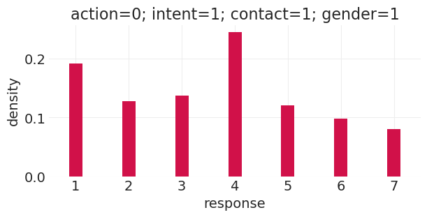
run_total_gender_counterfactual(action=0, intent=1, contact=1, gender=0)
Sampling: [response]
run_total_gender_counterfactual(action=0, intent=1, contact=1, gender=1)
Sampling: [response]
等一下!这是一个自愿样本。#
utils.draw_causal_graph(
    edge_list=[
        ("X", "R"),
        ("S", "R"),
        ("E", "R"),
        ("Y", "R"),
        ("G", "R"),
        ("Y", "E"),
        ("G", "E"),
        ("E", "P"),
        ("Y", "P"),
        ("G", "P"),
    ],
    node_props={
        "X": {"label": "action, intenition, contact, X"},
        "R": {"color": "red", "label": "response, R"},
        "S": {"label": "story, S"},
        "E": {"label": "education, E"},
        "Y": {"label": "age, Y"},
        "G": {"label": "gender, G"},
        "P": {"label": "participation, P", "color": "blue", "style": "dashed"},
        "unobserved": {"style": "dashed"},
    },
    edge_props={
        ("E", "P"): {"color": "blue"},
        ("Y", "P"): {"color": "blue"},
        ("G", "P"): {"color": "blue"},
        ("X", "R"): {"color": "red"},
    },
    graph_direction="LR",
)

自愿样本、参与和内生选择#
年龄、教育程度和性别都促成了一个未测量的变量:参与度
参与度是一个对撞机:条件化原因 E、Y、G 会共同变化
实际上不可能估计性别的总效应
我们可以估计按教育程度 \(E\) 和年龄 \(Y\) 分层后的性别 \(G\) 的直接效应
查看样本中教育程度和年龄的分布#
_, axs = plt.subplots(1, 2, figsize=(10, 3), gridspec_kw={"width_ratios": [2, 4]})

EDUCATION_ORDERED_LIST = [
    "Elementary School",
    "Middle School",
    "Some High School",
    "High School Graduate",
    "Some College",
    "Bachelor's Degree",
    "Master's Degree",
    "Graduate Degree",
]
EDUCUATION_MAP = {edu: ii + 1 for ii, edu in enumerate(EDUCATION_ORDERED_LIST)}
EDUCUATION_MAP_R = {v: k for k, v in EDUCUATION_MAP.items()}
TROLLEY["education_level"] = TROLLEY.edu.map(EDUCUATION_MAP)
TROLLEY["education"] = TROLLEY.education_level.map(EDUCUATION_MAP_R)


edu = TROLLEY.groupby("edu").count()[["case"]].rename(columns={"case": "count"})
edu.reset_index(inplace=True)
edu["edu_level"] = edu["edu"].map(EDUCUATION_MAP)

edu.sort_values("edu_level", inplace=True)

plt.sca(axs[0])
plt.bar(edu["edu_level"], edu["count"], width=0.25)
plt.xlabel("education level (ordered)")
plt.ylabel("frequency")
plt.title("education distribution")

plt.sca(axs[1])
age_counts = TROLLEY.groupby("age").count()
plt.bar(age_counts.index, age_counts.case, color="C1", width=0.8)
plt.xlabel("age (years)")
plt.title("age distribution");
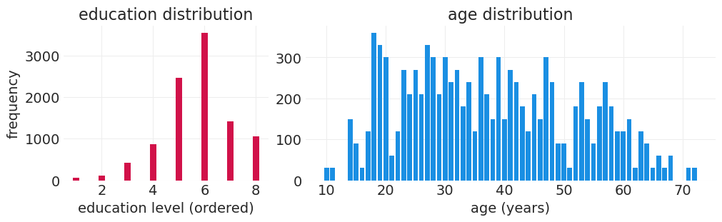
数据样本的教育程度和年龄分布与人口分布不一致的观察结果提供了证据,表明这些变量可能是与参与度相关的混杂因素。
有序单调预测变量#
与响应结果类似,教育程度也是一个有序类别。
每个级别对参与度/响应的影响不太可能相同
我们希望每个级别都有一个参数,同时强制排序,以便每个后续级别的影响幅度都大于前一个级别。
对于每个教育程度级别
(小学)\(\rightarrow \phi_i = 0\)
(中学)\(\rightarrow \phi_i = \delta_1\)
(部分高中)\(\rightarrow \phi_i = \delta_1 + \delta_2\)
(高中毕业)\(\rightarrow \phi_i = \delta_1 + \delta_2 + \delta_3\)
(部分大学)\(\rightarrow \phi_i = \delta_1 + \delta_2 + \delta_3 + \delta_4\)
(大学毕业)\(\rightarrow \phi_i = \delta_1 + \delta_2 + \delta_3 + \delta_4 + \delta_5\)
(硕士学位)\(\rightarrow \phi_i = \delta_1 + \delta_2 + \delta_3 + \delta_4 + \delta_5 + \delta_6\)
(研究生学位)\(\rightarrow \phi_i = \delta_1 + \delta_2 + \delta_3 + \delta_4 + \delta_5 + \delta_6+ \delta_7 = \beta_E\)
其中 \(\beta_E\) 是教育程度的最大效应。因此,我们将最大效应分解为教育程度项的凸组合。
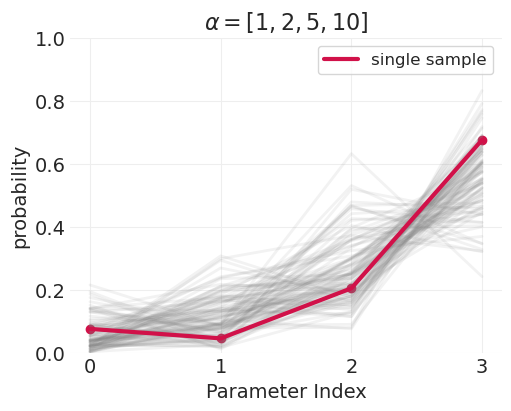
有序单调先验#
\(\delta\) 参数形成一个单纯形——比例向量,总和为 1
单纯形参数空间由 狄利克雷分布 建模
狄利克雷分布为我们提供了分布上的分布
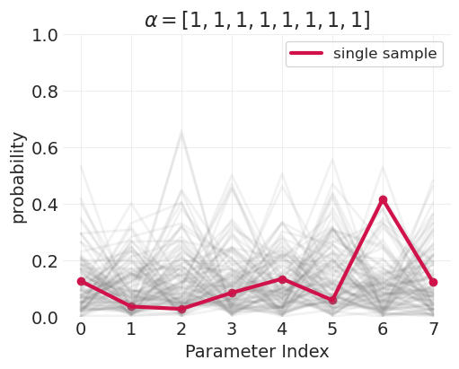
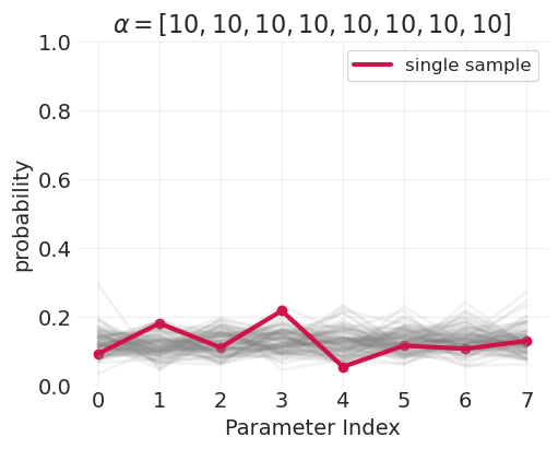
演示狄利克雷分布的参数化#
def plot_dirichlet(alpha, n_samples=100, ax=None, random_seed=123):
    """
    `alpha` is a vector of relative parameter importances. Larger
    values make the distribution more concentrated over the mean
    proportion.
    """
    np.random.seed(random_seed)
    if ax is not None:
        plt.sca(ax)
    else:
        _, ax = plt.subplots(figsize=(5, 4))
    dirichlet = stats.dirichlet(alpha)
    dirichlet_samples = dirichlet.rvs(size=n_samples).T
    plt.plot(dirichlet_samples, alpha=0.1, color="gray", linewidth=2)
    plt.plot(
        np.arange(len(alpha)),
        dirichlet_samples[:, 0],
        color="C0",
        linewidth=3,
        label="single sample",
    )
    plt.scatter(np.arange(len(alpha)), dirichlet_samples[:, 0], color="C0")

    plt.xticks(np.arange(len(alpha)))
    plt.xlabel("Parameter Index")
    plt.ylim([0, 1])
    plt.ylabel("probability")
    plt.title(f"$\\alpha={list(alpha)}$")
    plt.legend()


n_ordered_categories = 8
dirichlet_alphas = [
    np.ones(n_ordered_categories).astype(int),
    np.ones(n_ordered_categories).astype(int) * 10,
    np.round((1 + np.arange(4) ** 2), 1),
]

for alphas in dirichlet_alphas:
    plot_dirichlet(alphas)
评估教育程度的直接效应:按性别和年龄分层#
McElreath 在讲座中构建了一个性别总效应的模型,但随后指出,由于性别(通过参与度)造成的后门路径,我们无法解释教育程度的总原因。因此,我们需要也按性别分层。
# Add interaction of education level with gender to the dataset
EDUCATION_LEVEL_ID, EDUCATION_LEVEL = pd.factorize(TROLLEY.education_level, sort=True)
EDUCATION_LEVEL = [EDUCUATION_MAP_R[e] for e in EDUCATION_LEVEL]
N_EDUCATION_LEVELS = len(EDUCATION_LEVEL)

AGE = utils.standardize(TROLLEY.age.values)

DIRICHLET_PRIOR_WEIGHT = 2.0

coords = coords = {
    "GENDER": GENDER,
    "EDUCATION_LEVEL": EDUCATION_LEVEL,
    "CUTPOINTS": np.arange(1, N_RESPONSE_CLASSES).astype(int),
}

with pm.Model(coords=coords) as direct_effect_education_model:

    # Data for posterior predictions
    action = pm.Data("action", TROLLEY.action.astype(float))
    intent = pm.Data("intent", TROLLEY.intention.astype(float))
    contact = pm.Data("contact", TROLLEY.contact.astype(float))
    gender = pm.Data("gender", GENDER_ID)
    age = pm.Data("age", AGE)
    education_level = pm.Data("education_level", EDUCATION_LEVEL_ID)

    # Priors (all gender-level parameters)
    beta_action = pm.Normal("beta_action", 0, 0.5, dims="GENDER")
    beta_intent = pm.Normal("beta_intent", 0, 0.5, dims="GENDER")
    beta_contact = pm.Normal("beta_contact", 0, 0.5, dims="GENDER")
    beta_education = pm.Normal("beta_education", 0, 0.5, dims="GENDER")
    beta_age = pm.Normal("beta_age", 0, 0.5, dims="GENDER")

    # Education deltas_{j=1...|E|}.
    delta_dirichlet = pm.Dirichlet(
        "delta", np.ones(N_EDUCATION_LEVELS - 1) * DIRICHLET_PRIOR_WEIGHT
    )

    # Insert delta_0 = 0.0 at index 0 of parameter list
    delta_0 = [0.0]
    delta_education = pm.Deterministic(
        "delta_education", pm.math.concatenate([delta_0, delta_dirichlet]), dims="EDUCATION_LEVEL"
    )

    # For each level of education, the cumulative delta_E, phi_i
    cumulative_delta_education = delta_education.cumsum()

    # Response cut points
    cutpoints = pm.Normal(
        "alpha",
        mu=0,
        sigma=1,
        transform=pm.distributions.transforms.univariate_ordered,
        shape=N_RESPONSE_CLASSES - 1,
        initval=np.arange(N_RESPONSE_CLASSES - 1)
        - 2.5,  # use ordering (with coarse log-odds centering) for init
        dims="CUTPOINTS",
    )

    # Likelihood
    phi = (
        beta_education[gender] * cumulative_delta_education[education_level]
        + beta_age[gender] * age
        + beta_action[gender] * action
        + beta_intent[gender] * intent
        + beta_contact[gender] * contact
    )

    pm.OrderedLogistic("response", cutpoints=cutpoints, eta=phi, observed=RESPONSE_ID)

pm.model_to_graphviz(direct_effect_education_model)

with direct_effect_education_model:
    direct_effect_education_inference = pm.sample()
Initializing NUTS using jitter+adapt_diag...
Multiprocess sampling (4 chains in 4 jobs)
NUTS: [beta_action, beta_intent, beta_contact, beta_education, beta_age, delta, alpha]
Sampling 4 chains for 1_000 tune and 1_000 draw iterations (4_000 + 4_000 draws total) took 145 seconds.
az.summary(
    direct_effect_education_inference,
    var_names=[
        "alpha",
        "beta_action",
        "beta_intent",
        "beta_contact",
        "beta_education",
        "beta_age",
        "delta_education",
    ],
)
| 平均值 | 标准差 | hdi_3% | hdi_97% | mcse_mean | mcse_sd | ess_bulk | ess_tail | r_hat | |
|---|---|---|---|---|---|---|---|---|---|
| alpha[1] | -2.892 | 0.103 | -3.082 | -2.692 | 0.003 | 0.002 | 1474.0 | 2003.0 | 1.01 |
| alpha[2] | -2.208 | 0.101 | -2.404 | -2.023 | 0.003 | 0.002 | 1518.0 | 1899.0 | 1.01 |
| alpha[3] | -1.620 | 0.100 | -1.817 | -1.439 | 0.002 | 0.002 | 1648.0 | 1872.0 | 1.01 |
| alpha[4] | -0.579 | 0.098 | -0.775 | -0.402 | 0.002 | 0.002 | 1634.0 | 2087.0 | 1.01 |
| alpha[5] | 0.108 | 0.098 | -0.078 | 0.294 | 0.002 | 0.002 | 1628.0 | 2018.0 | 1.01 |
| alpha[6] | 1.037 | 0.100 | 0.833 | 1.212 | 0.002 | 0.002 | 1657.0 | 2151.0 | 1.01 |
| beta_action[F] | -0.559 | 0.059 | -0.673 | -0.454 | 0.001 | 0.001 | 3411.0 | 2829.0 | 1.00 |
| beta_action[M] | -0.807 | 0.054 | -0.905 | -0.701 | 0.001 | 0.001 | 3840.0 | 3128.0 | 1.00 |
| beta_intent[F] | -0.662 | 0.052 | -0.757 | -0.567 | 0.001 | 0.001 | 3929.0 | 3222.0 | 1.00 |
| beta_intent[M] | -0.756 | 0.049 | -0.849 | -0.663 | 0.001 | 0.001 | 3760.0 | 2364.0 | 1.00 |
| beta_contact[F] | -0.768 | 0.072 | -0.906 | -0.636 | 0.001 | 0.001 | 3835.0 | 3171.0 | 1.00 |
| beta_contact[M] | -1.092 | 0.067 | -1.218 | -0.962 | 0.001 | 0.001 | 3807.0 | 2790.0 | 1.00 |
| beta_education[F] | -0.629 | 0.132 | -0.889 | -0.383 | 0.003 | 0.002 | 1751.0 | 2265.0 | 1.00 |
| beta_education[M] | 0.407 | 0.132 | 0.169 | 0.660 | 0.003 | 0.002 | 1797.0 | 2180.0 | 1.00 |
| beta_age[F] | -0.001 | 0.028 | -0.049 | 0.054 | 0.000 | 0.000 | 3850.0 | 2987.0 | 1.00 |
| beta_age[M] | -0.133 | 0.028 | -0.185 | -0.079 | 0.001 | 0.000 | 2720.0 | 2807.0 | 1.00 |
| delta_education[小学] | 0.000 | 0.000 | 0.000 | 0.000 | 0.000 | 0.000 | 4000.0 | 4000.0 | NaN |
| delta_education[中学] | 0.152 | 0.089 | 0.009 | 0.309 | 0.001 | 0.001 | 3154.0 | 1911.0 | 1.00 |
| delta_education[部分高中] | 0.151 | 0.085 | 0.014 | 0.304 | 0.001 | 0.001 | 3338.0 | 2363.0 | 1.00 |
| delta_education[高中毕业] | 0.284 | 0.110 | 0.088 | 0.489 | 0.002 | 0.001 | 3164.0 | 1833.0 | 1.00 |
| delta_education[部分大学] | 0.080 | 0.051 | 0.001 | 0.172 | 0.001 | 0.001 | 3342.0 | 2077.0 | 1.00 |
| delta_education[学士学位] | 0.058 | 0.044 | 0.002 | 0.137 | 0.001 | 0.001 | 2334.0 | 2120.0 | 1.00 |
| delta_education[硕士学位] | 0.237 | 0.070 | 0.104 | 0.365 | 0.001 | 0.001 | 3256.0 | 2183.0 | 1.00 |
| delta_education[研究生学位] | 0.037 | 0.025 | 0.001 | 0.082 | 0.000 | 0.000 | 5157.0 | 3405.0 | 1.00 |
# Verify that education deltas are on the 8-simplex
assert np.isclose(
    az.summary(direct_effect_education_inference, var_names=["delta_education"])["mean"].sum(),
    1.0,
    atol=0.01,
)
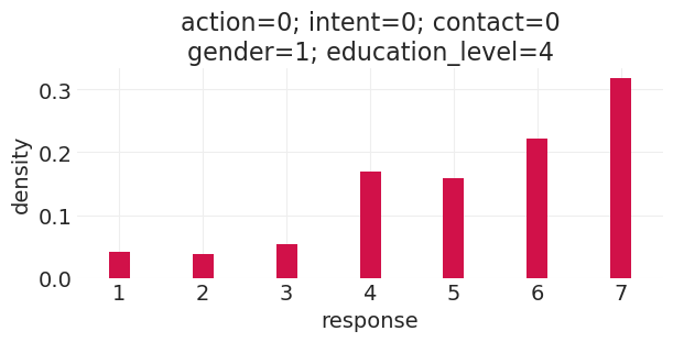
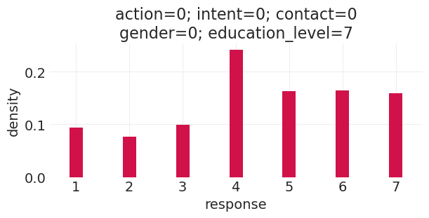
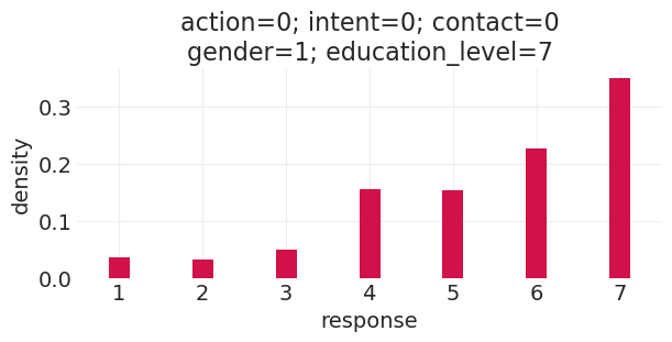
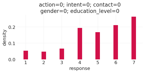
运行反事实#
def run_direct_education_counterfactual(
    action=0, intent=0, contact=0, gender=0, education_level=4, ax=None
):
    with direct_effect_education_model:
        pm.set_data(
            {
                "action": xr.DataArray([action] * N_TROLLEY_RESPONSES),
                "intent": xr.DataArray([intent] * N_TROLLEY_RESPONSES),
                "contact": xr.DataArray([contact] * N_TROLLEY_RESPONSES),
                "gender": xr.DataArray([gender] * N_TROLLEY_RESPONSES),
                "education_level": xr.DataArray([education_level] * N_TROLLEY_RESPONSES),
            }
        )
        ppd = pm.sample_posterior_predictive(
            direct_effect_education_inference, extend_inferencedata=False
        )

    # recode back to 1-7
    posterior_predictive = ppd.posterior_predictive["response"] + 1

    if ax is not None:
        plt.sca(ax)
    else:
        plt.subplots(figsize=(6, 3))

    counts, bins = np.histogram(posterior_predictive.values.ravel(), bins=np.arange(1, 9))
    total_counts = counts.sum()
    counts = [c / total_counts for c in counts]
    plt.bar(bins[:-1], counts, width=0.25)

    plt.xlim([0.5, 7.5])
    plt.xlabel("response")
    plt.ylabel("density")
    plt.title(
        f"action={action}; intent={intent}; contact={contact}\ngender={gender}; education_level={education_level}"
    )
run_direct_education_counterfactual(education_level=4, gender=0)
Sampling: [response]

run_direct_education_counterfactual(education_level=4, gender=1)
Sampling: [response]
run_direct_education_counterfactual(education_level=7, gender=0)
Sampling: [response]
run_direct_education_counterfactual(education_level=7, gender=1)
Sampling: [response]
run_direct_education_counterfactual(education_level=0, gender=0)
Sampling: [response]
run_direct_education_counterfactual(education_level=0, gender=1)
Sampling: [response]

复杂因果效应#
这里的一些教训是,复杂的因果图看起来工作量很大,但它允许我们
绘制显式的生成模型
绘制目标因果效应的显式估计量——我们需要识别正确的调整集
生成非线性因果关系和反事实的模拟——不要直接解释参数,生成预测
重复观察#
请注意,某些维度具有重复观察——例如,故事 ID 和响应者 ID。我们可以利用这些重复观察来估计未观察到的现象,例如个体响应偏差(类似于葡萄酒评委的区分水平)或故事偏差
奖励:描述和因果推断#
主要回顾之前的研究,技术说明不多。主要的观点是,描述(和预测)通常被认为与因果建模正交,但实际上在正确执行时涉及因果模型。
需要注意的事项#
高质量数据 > 更大数据
更大、有偏差的数据会放大偏差
更好的模型 > 平均值(XBox 投票)。更好的(因果)模型可以解决不具代表性的样本
事后分层
仍然影响描述性模型
没有原因输入;就没有描述输出
选择节点
可以纳入因果模型以捕捉非均匀参与
正确的行动取决于选择的原因
始终认真思考潜在的未建模的选择偏差
诚实的数字学术研究的 4 步计划#
确定我们试图描述什么
对此描述的理想数据是什么?
我们实际拥有什么数据?这几乎从不是 (2)。
(2)和(3)之间差异的原因是什么?
(可选)我们能否使用我们实际拥有的数据 (3) 和导致该数据的模型 (4) 来估计我们试图描述的内容 (1)
许可声明#
此示例 галерея 中的所有笔记本均根据 MIT 许可证 提供,该许可证允许修改和再分发以用于任何用途,前提是保留版权和许可声明。
引用 PyMC 示例#
要引用此笔记本,请使用 Zenodo 为 pymc-examples 存储库提供的 DOI。
重要提示
许多笔记本都改编自其他来源:博客、书籍…… 在这种情况下,您也应该引用原始来源。
还请记住引用您的代码使用的相关库。
这是一个 bibtex 中的引用模板
@incollection{citekey,
  author    = "<notebook authors, see above>",
  title     = "<notebook title>",
  editor    = "PyMC Team",
  booktitle = "PyMC examples",
  doi       = "10.5281/zenodo.5654871"
}
一旦呈现,它可能看起来像