


多层模型探险#
此笔记本是 PyMC 移植的 Statistical Rethinking 2023 系列讲座的一部分,由 Richard McElreath 讲授。
# Ignore warnings
import warnings

import arviz as az
import numpy as np
import pandas as pd
import pymc as pm
import statsmodels.formula.api as smf
import utils as utils
import xarray as xr

from matplotlib import pyplot as plt
from matplotlib import style
from scipy import stats as stats

warnings.filterwarnings("ignore")

# Set matplotlib style
STYLE = "statistical-rethinking-2023.mplstyle"
style.use(STYLE)
回顾:绘制贝叶斯猫头鹰 🦉#
确定 估计量
构建 科学模型(即因果模型),取决于 1。
使用 1 和 2 构建 统计模型
从 2 模拟 数据,并 验证 您可以从 3 中恢复
使用 3 分析真实数据。
在现实生活中,这绝不是一条线性路径;您像分支路径/选择你自己的冒险书一样,在 2-5 之间来回跳跃,迭代。
多层冒险#
同样,应用本课程中的方法也没有一种万能的方法。为了在应用这些方法时优化成功率,McElreath 提出了一些前进的策略(“路径”)
返回起点 – McElreath 建议回到课程的开始,复习您已经观察到大部分构建模块的材料。
事实证明,本仓库中提供的笔记是在课程的第三遍之后编写的。我再怎么强调都不过分,强烈建议您采纳 McElreath 的建议,从头开始复习这些材料。 材料很多,但我惊讶地发现,在这次讲座和之前的讲座之间的短暂时间内,我忘记了多少东西。同样,我也惊讶于第二次吸收这些材料变得容易得多——这真是对 McElreath 杰出的教学风格的证明。
略读和索引 – 不要纠结于细节,只需让自己熟悉可能性。
我发现有用的一件事是将课程中讨论的每个模型类编译成一个“食谱书”或“工具箱”,其中包含可重用于不同应用的即插即用模型
聚类 vs 特征#
聚类:数据中的子组(例如,坦克、参与者、故事、部门)
添加聚类相当简单
需要更多索引变量;更多总体先验
特征:模型的方面(即参数),因聚类而异(例如,生存率、平均响应率、录取率等)
添加特征需要更多复杂性
更多参数,特别是每个总体先验中的维度
可变效应作为混淆因素#
可变效应策略:使用重复观测和部分合并来估计聚类的未测量特征,这些特征在数据中留下了印记
预测视角:正则化
因果视角:未观测到的混淆因素令人恐惧,但利用重复观测为我们提供了更准确推断的希望
之前的示例:#
祖父母与教育#
utils.draw_causal_graph(
    edge_list=[("G", "P"), ("G", "C"), ("P", "C"), ("U", "P"), ("U", "C")],
    node_props={
        "G": {"label": "Grandparents Ed, G"},
        "P": {"label": "Parents Ed, P"},
        "C": {"label": "Children's Ed, C"},
        "U": {"label": "Neighborhood, U", "color": "blue"},
    },
    edge_props={("U", "P"): {"color": "blue"}, ("U", "C"): {"color": "blue"}},
)

社区是后门路径混淆因素,它阻止了 \(G\) 对 \(C\) 的直接效应的中介分析
但是,对于社区 U 进行重复观测使我们能够估计此混淆因素的影响
电车难题示例#
utils.draw_causal_graph(
    edge_list=[
        ("X", "R"),
        ("S", "R"),
        ("E", "R"),
        ("G", "R"),
        ("Y", "R"),
        ("U", "R"),
        ("G", "E"),
        ("Y", "E"),
        ("E", "P"),
        ("U", "P"),
    ],
    node_props={
        "X": {"label": "Treatment, X"},
        "R": {"label": "Response, R"},
        "P": {"label": "Participation, P", "style": "dashed"},
        "U": {"label": "Individual Traits, U", "color": "blue"},
        "unobserved": {"style": "dashed"},
    },
    edge_props={("U", "P"): {"color": "blue"}, ("U", "R"): {"color": "blue"}},
)

个体对响应尺度的反应各不相同,给我们的估计增加了噪音
然而,鉴于每个参与者都有重复观测,我们使用重复观测来估计这种噪音。
同样,个体特征可能会通过未观测到的参与节点导致抽样偏差;我们可以使用混合效应来帮助解决这种抽样偏差。
固定效应方法#
而不是部分合并,无合并。
使用固定效应而不是可变效应几乎没有好处。
例如,效率较低
专注于把故事讲清楚(生成模型、因果图),您可以稍后担心估计器效率等的细节
实践困难#
可变效应模型始终是一个好的默认选择,但是
如何使用多个聚类
预测现在处于层次结构的级别,我们关心哪个级别
抽样效率 – 例如,中心/非中心先验
群体层面混淆 – 例如,完全豪华贝叶斯或 Mundlak 机器。有关详细信息,请参阅 第 12 讲 - 多层模型的奖励章节
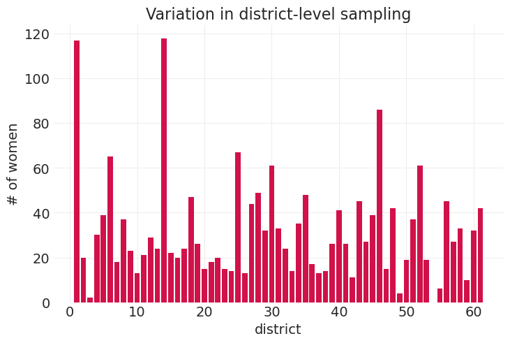
孟加拉国的生育率与行为#
1989 年生育率调查
1924 名女性,61 个地区
结局变量,\(C\): 避孕措施使用(二元变量)
预测变量:年龄,\(A\) 存活子女数 \(K\),城市/乡村地区 \(U\)
潜在的(未观测到的)混淆因素:家庭特征,\(F\)
地区 ID:\(D\)
FERTILITY = utils.load_data("bangladesh")
FERTILITY.head()
| woman | district | use.contraception | living.children | age.centered | urban | |
|---|---|---|---|---|---|---|
| 0 | 1 | 1 | 0 | 4 | 18.4400 | 1 |
| 1 | 2 | 1 | 0 | 1 | -5.5599 | 1 |
| 2 | 3 | 1 | 0 | 3 | 1.4400 | 1 |
| 3 | 4 | 1 | 0 | 4 | 8.4400 | 1 |
| 4 | 5 | 1 | 0 | 1 | -13.5590 | 1 |
竞争原因#
utils.draw_causal_graph(
    edge_list=[
        ("A", "C"),
        ("K", "C"),
        ("U", "C"),
        ("D", "C"),
        ("D", "U"),
        ("U", "K"),
        ("A", "K"),
        ("D", "K"),
        ("F", "C"),
        ("F", "K"),
    ],
    node_props={
        "A": {"label": "age, A"},
        "K": {"label": "# kids, K"},
        "U": {"label": "urbanity, U"},
        "D": {"label": "district, D"},
        "C": {"label": "contraceptive use, C"},
        "F": {"label": "family traits, F", "style": "dashed"},
        "unobserved": {"style": "dashed"},
    },
)

district_counts = FERTILITY.groupby("district").count()["woman"]
plt.bar(district_counts.index, district_counts)
plt.xlabel("district")
plt.ylabel("# of women")
plt.title("Variation in district-level sampling");
从简单开始:可变地区#
估计量:每个地区的避孕措施使用率;部分合并
模型:
每个地区的可变截距/偏移
utils.draw_causal_graph(
    edge_list=[
        ("D", "C"),
    ],
    node_props={
        "D": {"label": "district, D"},
        "C": {"label": "contraceptive use, C"},
    },
)

USES_CONTRACEPTION = FERTILITY["use.contraception"].values.astype(int)
DISTRICT_ID, _ = pd.factorize(FERTILITY.district)
DISTRICT = np.arange(1, 62).astype(
    int
)  # note: district 54 has no data so we create it's dim by hand

with pm.Model(coords={"district": DISTRICT}) as district_model:
    # Priors
    ## Global priors
    sigma = pm.Exponential("sigma", 1)  # variation amongst districts
    alpha_bar = pm.Normal("alpha_bar", 0, 1)  # the average district

    # District-level priors
    alpha = pm.Normal("alpha", alpha_bar, sigma, dims="district")

    # p(contraceptive)
    p_C = pm.Deterministic("p_C", pm.math.invlogit(alpha), dims="district")

    # Likelihood
    p = pm.math.invlogit(alpha[DISTRICT_ID])
    C = pm.Bernoulli("C", p=p, observed=USES_CONTRACEPTION)

    district_inference = pm.sample()
Initializing NUTS using jitter+adapt_diag...
Multiprocess sampling (4 chains in 4 jobs)
NUTS: [sigma, alpha_bar, alpha]
Sampling 4 chains for 1_000 tune and 1_000 draw iterations (4_000 + 4_000 draws total) took 3 seconds.
def plot_survival_posterior(
    inference,
    sigma=None,
    color="C0",
    var="p_C",
    hdi_prob=0.89,
    data_filter=None,
    title=None,
    ax=None,
):

    if ax is None:
        _, ax = plt.subplots(figsize=(10, 4))

    def reorder_missing_district_param(vec):
        """
        It appears that pymc tacks on the estimates for district with no data
        (54) onto the end of the parameter vector, so we put it into the correct
        position with this closure
        """
        vec_ = vec.copy()
        end = vec_[-1]  # no data is district 54 (index 53)
        vec_ = np.delete(vec_, -1)
        vec_ = np.insert(vec_, 52, end)
        return vec_

    # Filter the dataset for urban/rural if requested
    if data_filter == "urban":
        data_mask = (FERTILITY.urban).astype(bool)
    elif data_filter == "rural":
        data_mask = (1 - FERTILITY.urban).astype(bool)
    else:
        data_mask = np.ones(len(FERTILITY)).astype(bool)

    plot_data = FERTILITY[data_mask]
    district_counts = plot_data.groupby("district").count()["woman"]
    contraceptive_counts = plot_data.groupby("district").sum()["use.contraception"]
    proportion_contraceptive = contraceptive_counts / district_counts

    plt.sca(ax)
    utils.plot_scatter(
        xs=proportion_contraceptive.index,
        ys=proportion_contraceptive.values,
        color="k",
        s=50,
        zorder=3,
        alpha=0.8,
        label="raw proportions",
    )

    # Posterior per-district mean survival probability
    posterior_mean = inference.posterior.mean(dim=("chain", "draw"))[var]
    posterior_mean = reorder_missing_district_param(posterior_mean.values)

    utils.plot_scatter(
        DISTRICT, posterior_mean, color=color, zorder=50, alpha=0.8, label="posterior means"
    )

    # Posterior HDI error bars
    hdis = az.hdi(inference.posterior, var_names=var, hdi_prob=hdi_prob)[var].values

    error_upper = reorder_missing_district_param(hdis[:, 1]) - posterior_mean
    error_lower = posterior_mean - reorder_missing_district_param(hdis[:, 0])
    utils.plot_errorbar(
        xs=DISTRICT,
        ys=posterior_mean,
        error_lower=error_lower,
        error_upper=error_upper,
        colors=color,
        error_width=8,
    )

    # Add empirical mean
    empirical_mean = FERTILITY[data_mask]["use.contraception"].mean()
    plt.axhline(y=empirical_mean, c="k", linestyle="--", label="global mean")

    plt.ylim([-0.05, 1.05])
    plt.xlabel("district ")
    plt.ylabel("prob. use contraception")
    plt.title(title)
    plt.legend();
仅地区模型后验预测#
plot_survival_posterior(district_inference, title="District Model")
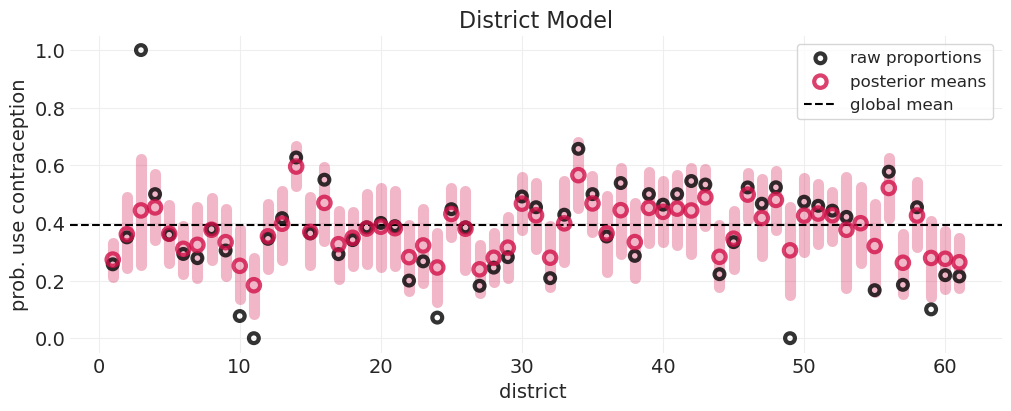
研究后验图#
样本量小的地区(例如地区 3)具有
较大的误差条 – 显示更多不确定性估计
表现出更多收缩
后验被拉向全局均值(虚线)
红色圆圈远离黑色圆圈)因为模型不太自信
样本量大的地区(例如地区 1)具有
较小的误差条 – 对估计的确定性更高
较少收缩
后验更接近该地区的经验观测
没有数据的地区(例如地区 49)仍然有后验
来自部分合并的信息后验
均值接近全局均值
误差条比其他地区大(看起来我的误差条代码中可能存在索引错误——需要调查一下)
可变地区 + 城市#
utils.draw_causal_graph(
    edge_list=[
        ("A", "C"),
        ("K", "C"),
        ("U", "C"),
        ("D", "C"),
        ("D", "U"),
        ("U", "K"),
        ("A", "K"),
        ("D", "K"),
    ],
    node_props={
        "A": {"color": "lightgray"},
        "K": {"color": "lightgray"},
    },
    edge_props={("A", "K"): {"color": "lightgray"}, ("A", "C"): {"color": "lightgray"}},
)

城市生活的影响是什么?
注意
地区特征具有潜在的群体层面混淆因素
\(U\) 的总效应通过 \(K\)
不要按 \(K\) 分层 – 这是一个对撞因子,它通过 \(D\) 打开了地区层面混淆
统计模型#
utils.draw_causal_graph(
    edge_list=[
        ("D", "C"),
        ("U", "C"),
    ],
    node_props={
        "D": {"label": "district, D"},
        "C": {"label": "contraceptive use, C"},
    },
)

拟合地区-城市模型#
我们在这里使用非中心化先验版本——有关非中心化的详细信息将在稍后讨论
URBAN_CODED, URBAN = pd.factorize(FERTILITY.urban, sort=True)

with pm.Model(coords={"district": DISTRICT}) as district_urban_model:

    # Mutable data
    urban = pm.Data("urban", URBAN_CODED)

    # Priors
    # District offset
    alpha_bar = pm.Normal("alpha_bar", 0, 1)  # the average district
    sigma = pm.Exponential("sigma", 1)  # variation amongst districts

    # Uncentered parameterization
    z_alpha = pm.Normal("z_alpha", 0, 1, dims="district")
    alpha = alpha_bar + z_alpha * sigma

    # District / urban interaction
    beta_bar = pm.Normal("beta_bar", 0, 1)  # the average urban effect
    tau = pm.Exponential("tau", 1)  # variation amongst urban

    # Uncentered parameterization
    z_beta = pm.Normal("z_beta", 0, 1, dims="district")
    beta = beta_bar + z_beta * tau

    # Recored p(contraceptive)
    p_C = pm.Deterministic("p_C", pm.math.invlogit(alpha + beta))
    p_C_urban = pm.Deterministic("p_C_urban", pm.math.invlogit(alpha + beta))
    p_C_rural = pm.Deterministic("p_C_rural", pm.math.invlogit(alpha))

    # Likelihood
    p = pm.math.invlogit(alpha[DISTRICT_ID] + beta[DISTRICT_ID] * urban)
    C = pm.Bernoulli("C", p=p, observed=USES_CONTRACEPTION)

    district_urban_inference = pm.sample(target_accept=0.95)
Initializing NUTS using jitter+adapt_diag...
Multiprocess sampling (4 chains in 4 jobs)
NUTS: [alpha_bar, sigma, z_alpha, beta_bar, tau, z_beta]
Sampling 4 chains for 1_000 tune and 1_000 draw iterations (4_000 + 4_000 draws total) took 9 seconds.
总结城市-地区后验#
az.summary(district_urban_inference, var_names=["alpha_bar", "beta_bar", "tau", "sigma"])
| mean | sd | hdi_3% | hdi_97% | mcse_mean | mcse_sd | ess_bulk | ess_tail | r_hat | |
|---|---|---|---|---|---|---|---|---|---|
| alpha_bar | -0.702 | 0.090 | -0.869 | -0.533 | 0.002 | 0.001 | 3586.0 | 3206.0 | 1.00 |
| beta_bar | 0.620 | 0.151 | 0.341 | 0.909 | 0.002 | 0.001 | 5350.0 | 3183.0 | 1.00 |
| tau | 0.543 | 0.212 | 0.135 | 0.953 | 0.007 | 0.005 | 1014.0 | 1022.0 | 1.01 |
| sigma | 0.487 | 0.087 | 0.329 | 0.645 | 0.002 | 0.001 | 1856.0 | 2535.0 | 1.00 |
比较城市/乡村形式的后验预测,单模型联合拟合#
fig, axs = plt.subplots(2, 1, figsize=(10, 8))
for ii, (label, var) in enumerate(zip(["rural", "urban"], ["p_C_rural", "p_C_urban"])):
    plot_survival_posterior(
        district_urban_inference, color=f"C{ii}", var=var, data_filter=label, ax=axs[ii]
    )
    plt.title(label)

# Save fig for reference in next lecture
utils.savefig("fertility_posterior_means_rural_urban.png")
saving figure to images/fertility_posterior_means_rural_urban.png
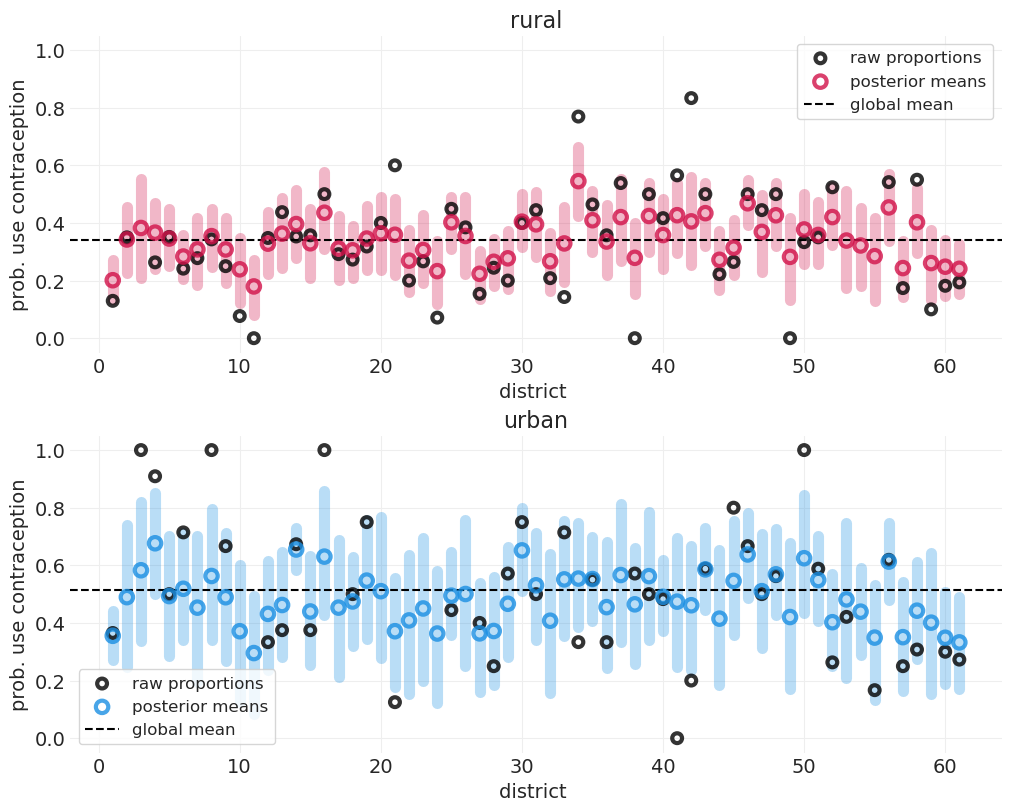
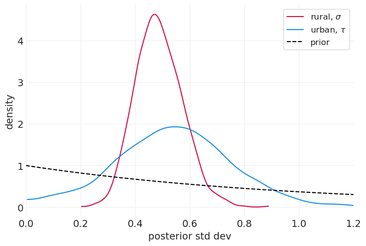
后验方差#
以上图表表明城市地区具有
更高的避孕措施使用总体比率
城市地区误差范围方差较高
下图再次确认,城市地区的避孕措施使用方差确实较大;城市地区的后验标准差参数 \(\tau\) 大于乡村地区的参数 \(\sigma\)
for ii, (label, var) in enumerate(zip(["rural, $\\sigma$", "urban, $\\tau$"], ["sigma", "tau"])):
    az.plot_dist(district_urban_inference.posterior[var], color=f"C{ii}", label=label)


def exponential_prior(x, lambda_=1):
    return lambda_ * np.exp(-lambda_ * x)


xs = np.linspace(0, 1.2)
plt.plot(xs, exponential_prior(xs), label="prior", color="k", linestyle="--")
plt.xlim([0, 1.2])
plt.xlabel("posterior std dev")
plt.ylabel("density")
plt.legend();
城市和乡村结果呈正相关#
posterior_mean = district_urban_inference.posterior.mean(dim=("chain", "draw"))
utils.plot_scatter(
    posterior_mean["p_C_rural"], posterior_mean["p_C_urban"], color="C0", label="posterior means"
)
correlation = np.corrcoef(posterior_mean["p_C_rural"], posterior_mean["p_C_urban"])[0][1]
plt.axvline(0.5, color="gray", linestyle="dashed")
plt.axhline(0.5, color="gray", linestyle="dashed")
plt.xlabel("prob C (rural)")
plt.ylabel("prob C (urban)")
plt.title(f"Correlation: {correlation:1.2f}")
plt.legend()
plt.axis("square")

# Save fig for reference in next lecture
utils.savefig("fertility_p_C_rural_urban.png");
saving figure to images/fertility_p_C_rural_urban.png
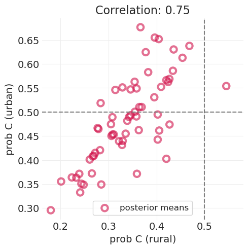
一些观察#
城市地区的避孕措施使用率高于乡村地区——大多数点都位于垂直线的左侧
每个地区的乡村和城市地区的避孕措施使用率之间存在高度相关性 (cc>0.7)。
我们应该能够利用这种相关性信息来做出更好的估计。更多内容即将推出!
总结:多层模型探险#
聚类:数据中独特的组
特征:模型的方面(例如参数),因聚类而异
有用的信息在特征之间传递
我们可以使用部分合并来有效估计特征,即使在缺乏数据的情况下也是如此
许可声明#
此示例库中的所有笔记本均根据 MIT 许可证 提供,该许可证允许修改和再分发用于任何用途,前提是版权和许可声明得到保留。
引用 PyMC 示例#
要引用此笔记本,请使用 Zenodo 为 pymc-examples 仓库提供的 DOI。
重要提示
许多笔记本改编自其他来源:博客、书籍…… 在这种情况下,您也应该引用原始来源。
另请记住引用您的代码使用的相关库。
这是一个 bibtex 中的引用模板
@incollection{citekey,
  author    = "<notebook authors, see above>",
  title     = "<notebook title>",
  editor    = "PyMC Team",
  booktitle = "PyMC examples",
  doi       = "10.5281/zenodo.5654871"
}
渲染后可能看起来像