


孟加拉国生育率再探#
utils.draw_causal_graph(
    edge_list=[
        ("A", "C"),
        ("K", "C"),
        ("U", "C"),
        ("D", "C"),
        ("D", "U"),
        ("U", "K"),
        ("A", "K"),
        ("D", "K"),
    ]
)

估计量 1:每个地区 \(D\) 的避孕药具使用率 \(C\)
估计量 2:“城市化”的影响 \(U\)
估计量 3:孩子数量 \(K\) 和年龄 \(A\) 的影响
地区是聚类#
农村/城市细分#
下面我们展示了农村地区(仅包括地区级截距 \(\alpha_{D[i]}\))与城市地区(包括城市地区的额外截距 \(\beta_{D[i]}\))组的避孕药具使用率。这些图是在 第 13 讲 - 多层冒险 中生成的。
utils.display_image("fertility_posterior_means_rural_urban.png", width=1000)
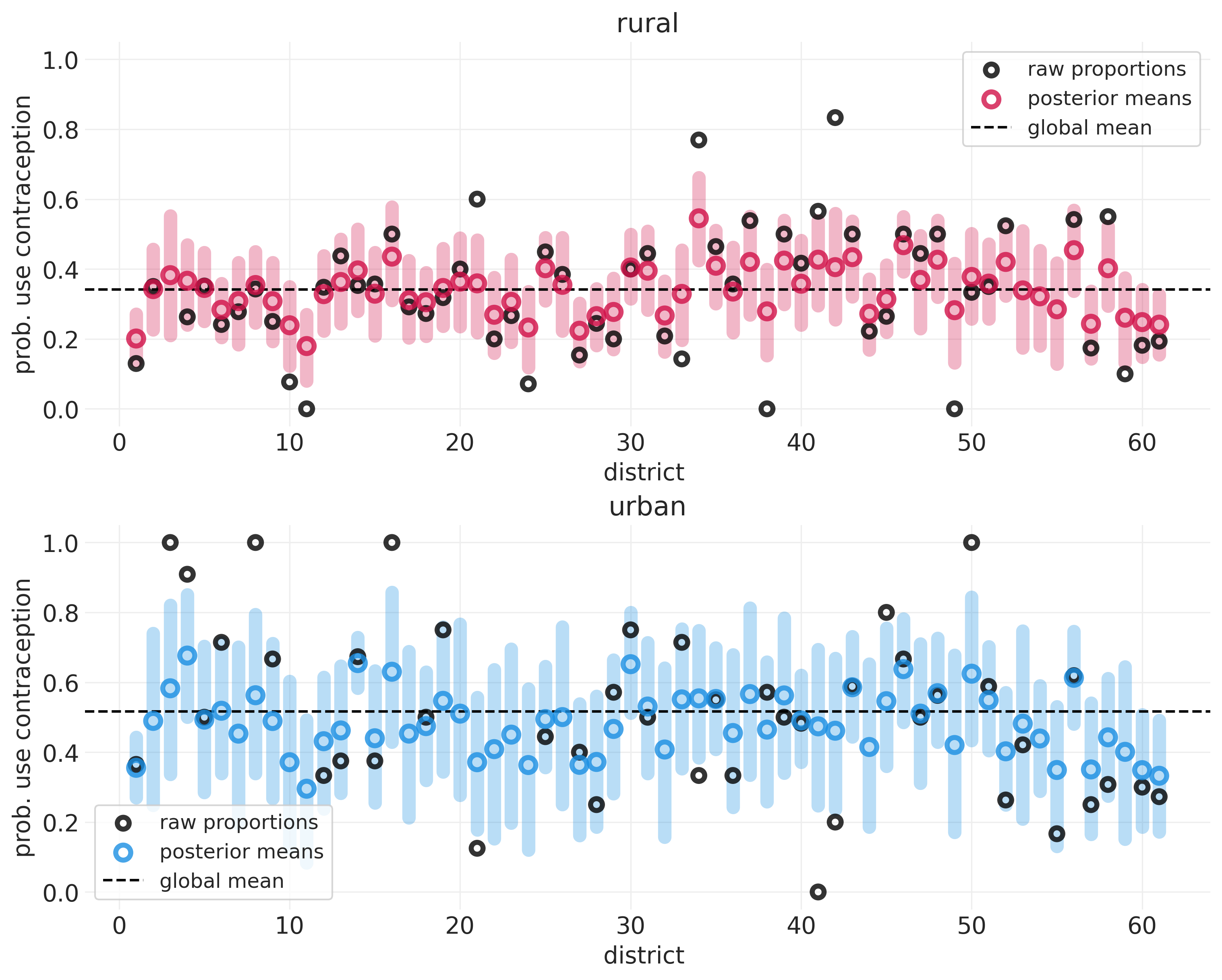
该图显示
平均而言,农村人口比城市地区人口更不可能使用避孕措施
顶部图中的虚线低于底部图中的虚线
城市样本较少,因此城市地区的不确定性范围较大
与农村地区相比,与城市人口相关的误差蓝色条更大,农村地区采样的民意调查更多。
城市化是一个相关特征#
下面我们绘制了城市地区 \(p(C | U=1)\) 与农村地区 \(p(C|U=0)\) 的避孕药具使用概率。这些图是在 第 13 讲 - 多层冒险 中生成的。
utils.display_image("fertility_p_C_rural_urban.png")
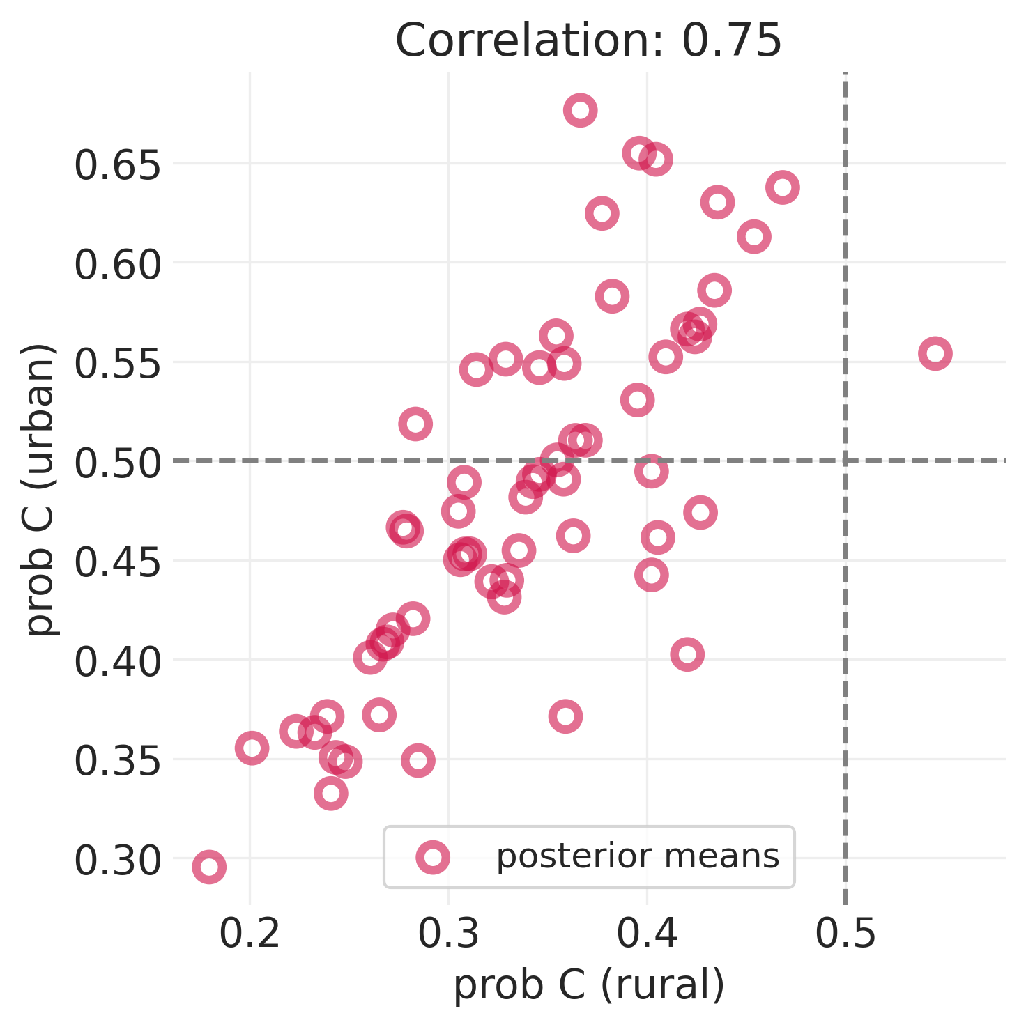
该图显示,城市/农村观察之间的避孕药具使用率是相关的 (cc>0.7)
🤔#
如果我们知道农村地区的避孕药具使用率,由于这种相关性,您可以更好地猜测城市地区的避孕药具使用率
我们没有让 Golem(即我们的统计模型)利用这种特征相关性,因此是在浪费信息
本讲座的重点是构建可以捕获特征之间相关信息的统计模型。
通过跨特征的部分合并,使推断更有效
估计相关性和部分合并演示
McElreath 继续展示了贝叶斯更新在具有相关特征的模型中的演示。它非常棒,我建议多次回顾该演示,但我太懒了,无法实现它(也没有聪明到在没有动画的情况下做到这一点,我正在尝试避免动画)。它将添加到 TODO 列表中。
添加相关特征#
每个聚类/子组的一个先验分布 \(\rightarrow a_j \sim \text{Normal}(\bar a , \sigma)\);允许部分合并
如果一个特征,则一维先验
\(a_j \sim \text{Normal}(\bar a, \sigma)\)
N 个特征的 N 维分布
我们使用特征的联合分布,而不是独立的分布(就像我们在之前的讲座中所做的那样)
\(a_{j, 1..N} \sim \text{MVNormal}(A, \Sigma)\)
例如,\([\alpha_j, \beta_j] \sim \text{MVNormal}([\bar \alpha, \bar \beta], \Sigma_{\alpha, \beta})\)
难点:学习特征之间的关联/相关性
“估计均值很容易”
“估计标准差很难”
“估计相关性非常难”
也就是说,通常尝试学习相关性是个好主意
如果您没有足够的样本/信号,您将退回到先验
之前的模型 – 使用不相关的城市特征#
utils.draw_causal_graph(
    edge_list=[
        ("A", "C"),
        ("K", "C"),
        ("U", "C"),
        ("D", "C"),
        ("D", "U"),
        ("U", "K"),
        ("A", "K"),
        ("D", "K"),
    ],
    node_props={"U": {"color": "red"}, "D": {"color": "red"}, "C": {"color": "red"}},
    edge_props={
        ("U", "K"): {"color": "red"},
        ("U", "C"): {"color": "red"},
        ("K", "C"): {"color": "red"},
    },
)

这是未居中的实现,或多或少从之前的讲座中复制粘贴而来
FERTILITY = utils.load_data("bangladesh")

USES_CONTRACEPTION = FERTILITY["use.contraception"].values.astype(int)
DISTRICT_ID, _ = pd.factorize(FERTILITY.district)
DISTRICT = np.arange(1, 62).astype(
    int
)  # note: district 54 has no data so we create it's dim by hand
URBAN_ID, URBAN = pd.factorize(FERTILITY.urban, sort=True)

with pm.Model(coords={"district": DISTRICT}) as uncorrelated_model:

    # Mutable data
    urban = pm.Data("urban", URBAN_ID)

    # Priors -- priors for $\alpha$ and $\beta$ are separate, independent Normal distributions
    # District offset
    alpha_bar = pm.Normal("alpha_bar", 0, 1)  # the average district
    sigma = pm.Exponential("sigma", 1)  # variation amongst districts

    # Uncentered parameterization
    z_alpha = pm.Normal("z_alpha", 0, 1, dims="district")
    alpha = pm.Deterministic("alpha", alpha_bar + z_alpha * sigma, dims="district")

    # District / urban interaction
    beta_bar = pm.Normal("beta_bar", 0, 1)  # the average urban effect
    tau = pm.Exponential("tau", 1)  # variation amongst urban

    # Uncentered parameterization
    z_beta = pm.Normal("z_beta", 0, 1, dims="district")
    beta = pm.Deterministic("beta", beta_bar + z_beta * tau, dims="district")

    # Recored p(contraceptive)
    p_C = pm.Deterministic("p_C", pm.math.invlogit(alpha + beta))
    p_C_urban = pm.Deterministic("p_C_urban", pm.math.invlogit(alpha + beta))
    p_C_rural = pm.Deterministic("p_C_rural", pm.math.invlogit(alpha))

    # Likelihood
    p = pm.math.invlogit(alpha[DISTRICT_ID] + beta[DISTRICT_ID] * urban)
    C = pm.Bernoulli("C", p=p, observed=USES_CONTRACEPTION)

    uncorrelated_inference = pm.sample(target_accept=0.95)
Initializing NUTS using jitter+adapt_diag...
Multiprocess sampling (4 chains in 4 jobs)
NUTS: [alpha_bar, sigma, z_alpha, beta_bar, tau, z_beta]
Sampling 4 chains for 1_000 tune and 1_000 draw iterations (4_000 + 4_000 draws total) took 10 seconds.
证明特征先验在不相关模型中是独立的#
下面我们从先验中采样,并表明所有地区的 \(\alpha\) 和 \(\beta\) 参数都与基轴对齐,表明没有相关性
def plot_2d_guassian_ci(R, mean=[0, 0], std=[1, 1], ci_prob=0.89, **plot_kwargs):
    """
    Plot the `ci_prob`% confidence interval for a 2D Gaussian defined
    by correlation matrix `R`, center `mean`, and standard deviations
    `std` along the marginals.
    """
    # Create a circle
    angles = np.linspace(0, 2 * np.pi, 100)
    radius = stats.norm.ppf(ci_prob)
    circle = radius * np.vstack([np.cos(angles), np.sin(angles)])

    # Warp circle using the covariance matrix
    D = np.diag(std)
    cov = D @ R @ D
    ellipse = sqrtm(np.matrix(cov)) @ circle
    plt.plot(ellipse[0] + mean[0], ellipse[1] + mean[1], linewidth=3, **plot_kwargs)
with uncorrelated_model:
    prior_pred = pm.sample_prior_predictive()

districts = [1, 10, 30, 61]
n_districts = len(districts)
fig, axs = plt.subplots(n_districts, 1, figsize=(6, n_districts * 4))
for ii, district in enumerate(districts):
    district_prior = prior_pred.prior.sel(district=district)
    plt.sca(axs[ii])
    az.plot_dist(
        district_prior["alpha"],
        district_prior["beta"],
        ax=axs[ii],
        contourf_kwargs={"cmap": "Reds"},
    )
    plt.xlim([-4, 4])
    plt.ylim([-4, 4])
    plt.xlabel("$\\alpha$")
    plt.ylabel("$\\beta$")
    plt.title(f"District {district} Prior")
Sampling: [C, alpha_bar, beta_bar, sigma, tau, z_alpha, z_beta]
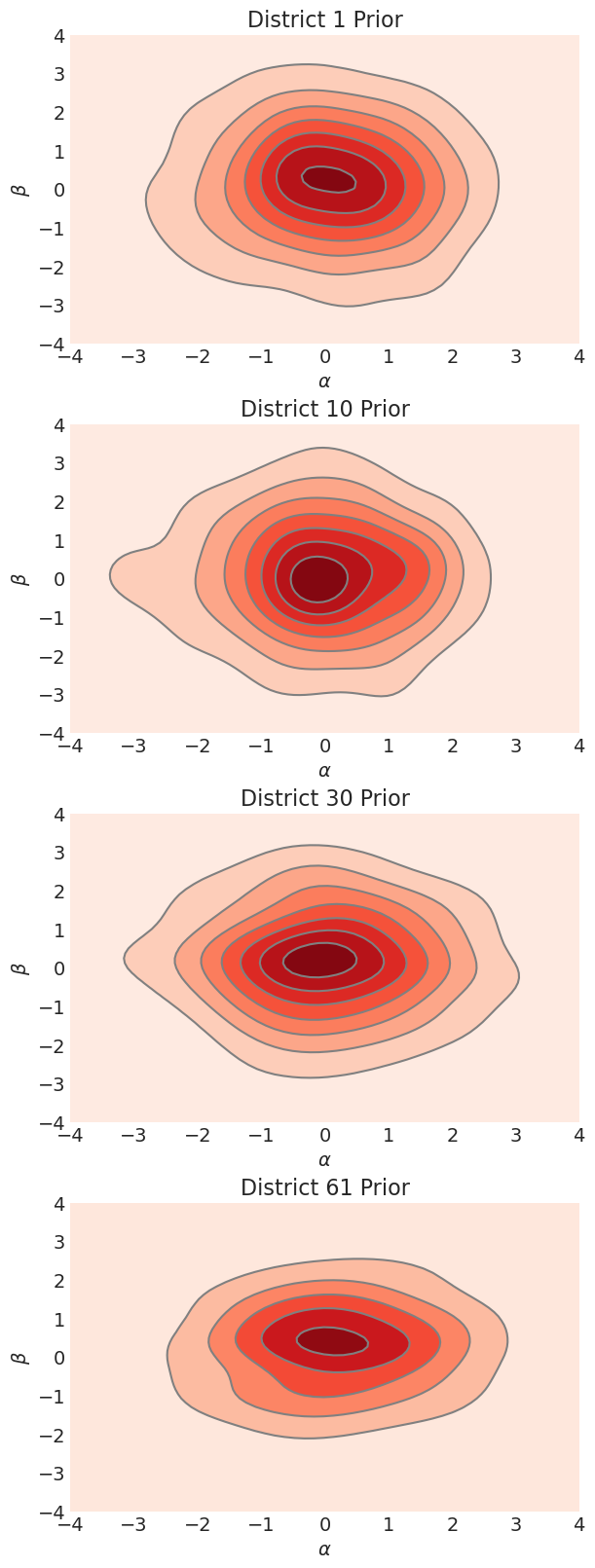
上面我们可以看到不相关模型提供的先验。我们可以判断它们是不相关的,因为
分布的主轴垂直于参数值的轴。
即,PDF 轮廓没有“倾斜”
多元正态先验#
来自多元先验的样本#
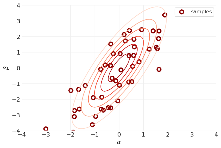
np.random.seed(123)
sigma = 1.0
tau = 2.0
R = np.array([[1, 0.8], [0.8, 1]])  # correlation matrix


stds = np.array([sigma, tau])
D = np.diag(stds)
Sigma = D @ R @ D  # convert correlation matrix to covariance matrix
mvnorm = stats.multivariate_normal(cov=Sigma)


def mvn_norm_pdf(
    xs,
    ys,
):
    return mvnorm.pdf(np.vstack([xs, ys]).T)


RESOLUTION = 100
xs = ys = np.linspace(-4, 4, RESOLUTION)
utils.plot_2d_function(xs, ys, mvn_norm_pdf, cmap="Reds")

n_samples = 50
samples = mvnorm.rvs(n_samples)
utils.plot_scatter(samples[:, 0], samples[:, 1], color="darkred", alpha=1, label="samples")
plt.xlabel("$\\alpha$")
plt.ylabel("$\\beta$")
plt.xlim([-4, 4])
plt.ylim([-4, 4])
plt.legend()

print(f"Standard deviations\n{stds}")
print(f"Correlation Matrix\n{R}")
print(f"Covariance Matrix\n{Sigma}")
print(f"Cholesky Matrix\n{np.linalg.cholesky(Sigma)}")
Standard deviations
[1. 2.]
Correlation Matrix
[[1.  0.8]
 [0.8 1. ]]
Covariance Matrix
[[1.  1.6]
 [1.6 4. ]]
Cholesky Matrix
[[1.  0. ]
 [1.6 1.2]]
具有相关城市特征的模型#
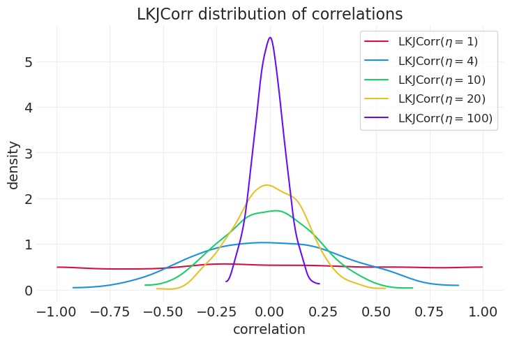
关于 LKJCorr 先验#
以 Lewandowski-Kurowicka-Joe 命名,他们是关于该分布的原始论文的作者
相关矩阵的先验
采用形状参数 \(\eta>0\)
\(\eta=1\) 会导致相关矩阵上的均匀分布
\(\eta \rightarrow \infty\),R 接近单位矩阵
更改相关矩阵的分布
etas = [1, 4, 10, 20, 100]
for ii, eta in enumerate(etas):
    rv = pm.LKJCorr.dist(n=2, eta=eta)
    samples = pm.draw(rv, 1000)
    az.plot_dist(samples, color=f"C{ii}", label=f"LKJCorr$(\\eta={eta})$")
plt.legend()
plt.xlabel("correlation")
plt.ylabel("density")
plt.title("LKJCorr distribution of correlations");
从 LKJCorr 采样的相关矩阵#
import matplotlib.transforms as transforms

from matplotlib.patches import Ellipse
from scipy.linalg import sqrtm


def sample_correlation_matrix_LKJ(dim=2, eta=4, n_samples=1):

    # Samples; LKJCorr returns correlations are returned as
    # upper-triangular matrix entries
    rv = pm.LKJCorr.dist(n=dim, eta=eta)
    samples = pm.draw(rv, n_samples)

    # Convert upper triangular entries to full correlation matrices
    # (there's likely a way to vectorize this, but meh it's a demo)
    covs = []
    upper_idx = np.triu_indices(n=dim, k=1)
    for sample in samples:
        cov = np.eye(dim) * 0.5
        cov[upper_idx[0], upper_idx[1]] = sample
        cov += cov.T
        covs.append(cov)
    return np.array(covs)


def sample_LKJCorr_prior(eta=1, n_samples=20, ax=None):
    plt.sca(ax)
    for _ in range(n_samples):

        R = sample_correlation_matrix_LKJ(eta=eta)

        # Sample a random standard deviation along each dimension
        std = stats.expon(0.1).rvs(2)  # exponential
        # std = np.random.rand(2) * 10  # uniform
        # std = np.abs(np.random.randn(2))  # half-normal

        plot_2d_guassian_ci(R, std=std, color="C0", alpha=0.25)

    plt.xlim([-2, 2])
    plt.ylim([-2, 2])
    plt.xlabel("$\\alpha$")
    plt.ylabel("$\\beta$")
    plt.title(f"Random Correlations Sampled\nfrom LKJCorr({eta}) prior");
etas = [1, 4, 10, 1000]
n_etas = len(etas)
_, axs = plt.subplots(n_etas, 1, figsize=(6, 6 * n_etas))
for ii, eta in enumerate(etas):
    sample_LKJCorr_prior(eta=eta, ax=axs[ii])
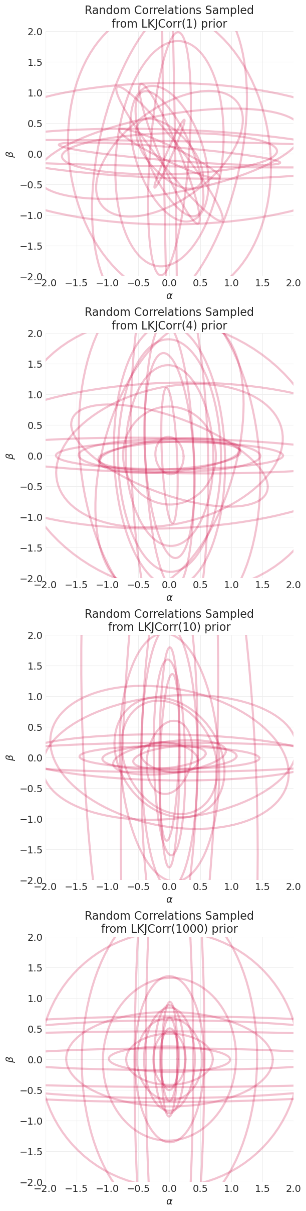
我们可以看到,随着 \(\eta\) 变得更大,相关矩阵的轴与参数空间的轴变得更加对齐,从而提供对角协方差样本
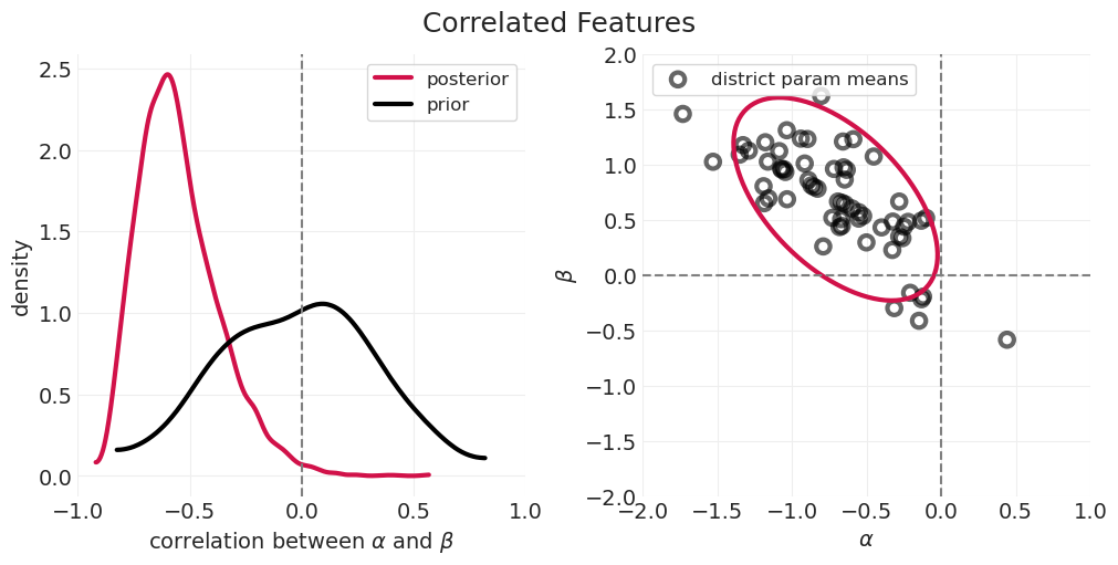
分析特征相关性#
correlated_posterior_mean = correlated_inference.posterior.mean(dim=("chain", "draw"))
print(f"Feature Covariance\n", correlated_posterior_mean["feature_cov"].values)
print(f"Feature Correlation\n", correlated_posterior_mean["feature_corr"].values)
print(f"Feature Std\n", correlated_posterior_mean["feature_std"].values)
Feature Covariance
 [[ 0.32032104 -0.24587394]
 [-0.24587394  0.60162453]]
Feature Correlation
 [[ 1.         -0.55103506]
 [-0.55103506  1.        ]]
Feature Std
 [0.55748164 0.74948169]
与先验比较#
with correlated_model:
    # Add prior samples
    correlated_prior_predictive = pm.sample_prior_predictive()
Sampling: [C, Rho, alpha_bar, beta_bar, z]
def plot_posterior_mean_alpha_beta(posterior_mean, title=None):
    alphas = posterior_mean["alpha"].values
    betas = posterior_mean["beta"].values
    alpha_mean = posterior_mean["alpha"].mean().values
    beta_mean = posterior_mean["beta"].mean().values

    # Correlated feature params
    if "feature_corr" in posterior_mean:
        posterior_R = posterior_mean["feature_corr"].values
        posterior_std = posterior_mean["feature_std"].values

    # Independent feature params
    else:
        cc = np.corrcoef(alphas, betas)[0][1]
        posterior_R = np.array([[1, cc], [cc, 1]])
        posterior_std = np.array([posterior_mean["sigma"], posterior_mean["tau"]])

    plot_2d_guassian_ci(R=posterior_R, mean=(alpha_mean, beta_mean), std=posterior_std, color="C0")

    utils.plot_scatter(
        xs=posterior_mean["alpha"],
        ys=posterior_mean["beta"],
        color="k",
        label="district param means",
    )

    plt.axvline(0, color="gray", linestyle="--")
    plt.axhline(0, color="gray", linestyle="--")
    plt.xlim([-2, 1])
    plt.ylim([-2, 2])
    plt.xlabel("$\\alpha$")
    plt.ylabel("$\\beta$")
    plt.legend()
    plt.title(title)


_, axs = plt.subplots(1, 2, figsize=(10, 5))

# Plot correlation distribution for posterior and prior
plt.sca(axs[0])
plot_kwargs = {"linewidth": 3}
az.plot_dist(
    correlated_inference.posterior["feature_corr"][:, :, 0, 1],
    label="posterior",
    plot_kwargs=plot_kwargs,
    ax=axs[0],
)
az.plot_dist(
    correlated_prior_predictive.prior["feature_corr"][:, :, 0, 1],
    color="k",
    label="prior",
    plot_kwargs=plot_kwargs,
    ax=axs[0],
)

plt.axvline(0, color="gray", linestyle="--")
plt.xlim([-1, 1])
plt.xlabel("correlation between $\\alpha$ and $\\beta$")
plt.ylabel("density")
plt.legend()

plt.sca(axs[1])

plot_posterior_mean_alpha_beta(correlated_posterior_mean)
plt.suptitle("Correlated Features", fontsize=18);
uncorrelated_posterior_mean = uncorrelated_inference.posterior.mean(dim=("chain", "draw"))

_, axs = plt.subplots(1, 2, figsize=(10, 5))

plt.sca(axs[0])
plot_posterior_mean_alpha_beta(uncorrelated_posterior_mean, title="uncorrelated features")

plt.sca(axs[1])
plot_posterior_mean_alpha_beta(correlated_posterior_mean, title="correlated features")
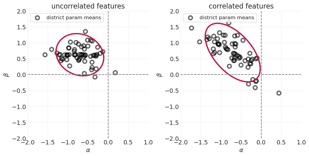
与不建模特征相关性的模型相比:具有不相关特征的模型表现出弱得多的负相关性(即,左侧的红色椭圆“向下倾斜”的程度较小)。
在结果尺度上比较模型。#
def plot_p_C_district_rural_urban(posterior_mean, title=None):
    for ii, (label, p_C) in enumerate(zip(["rural", "urban"], ["p_C_rural", "p_C_urban"])):
        color = f"C{ii}"
        plot_data = posterior_mean[p_C]
        utils.plot_scatter(DISTRICT, plot_data, label=label, color=color, alpha=0.8)

        # Add quantile indicators
        ql, median, qu = np.quantile(plot_data, [0.25, 0.5, 0.975])
        error = np.array((median - ql, qu - median))[:, None]
        plt.errorbar(
            x=0,
            y=median,
            yerr=error,
            color=color,
            capsize=5,
            linewidth=2,
            label=f"95%IPR:({ql:0.2f}, {qu:0.2f}))",
        )
        plt.axhline(median, color=color)

    plt.axhline(0.5, color="gray", linestyle="--", label="p=0.5")
    plt.legend(loc="upper right")
    plt.ylim([0, 1])
    plt.xlabel("district")
    plt.ylabel("prob. contraceptive use")
    plt.title(title)


_, axs = plt.subplots(2, 1, figsize=(10, 8))

plt.sca(axs[0])
plot_p_C_district_rural_urban(correlated_posterior_mean, title="correlated features")

plt.sca(axs[1])
plot_p_C_district_rural_urban(uncorrelated_posterior_mean, title="uncorrelated features")
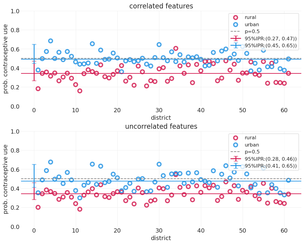
建模特征相关性允许城市地区以不同的方式捕获城市方差。虽然效果很微妙,但相关特征模型(顶部)表现出比不相关特征模型(0.41-0.65)更小的内百分位数范围 (IPR) (0.45-0.65)。
⚠️ 这实际上与讲座中报告的相反。我的直觉是,后验变异性会更小,因为我们正在跨特征共享信息,从而降低了我们的不确定性。但我很容易在这里做错或理解错误。
查看结果空间#
def plot_pC_rural_urban_xy(posterior_mean, label, color):
    utils.plot_scatter(
        xs=posterior_mean["p_C_rural"],
        ys=posterior_mean["p_C_urban"],
        label=label,
        color=color,
        alpha=0.8,
    )

    plt.axhline(0.5, color="gray", linestyle="--")
    plt.axvline(0.5, color="gray", linestyle="--")
    plt.xlabel("$p(C)$ (rural)")
    plt.ylabel("$p(C)$ (urban)")
    plt.legend()
    plt.axis("square")


def plot_pC_xy_movement(posterior_mean_a, posterior_mean_b):
    xs_a = posterior_mean_a["p_C_rural"]
    xs_b = posterior_mean_b["p_C_rural"]
    ys_a = posterior_mean_a["p_C_urban"]
    ys_b = posterior_mean_b["p_C_urban"]

    for ii, (xa, xb, ya, yb) in enumerate(zip(xs_a, xs_b, ys_a, ys_b)):
        label = "$p(C) $ change" if not ii else None
        plt.plot((xa, xb), (ya, yb), linewidth=0.5, color="C0", label=label)
    plt.legend(loc="upper left")


plot_pC_rural_urban_xy(uncorrelated_posterior_mean, label="uncorrelated features", color="k")
plot_pC_rural_urban_xy(correlated_posterior_mean, label="correlated features", color="C0")
plot_pC_xy_movement(uncorrelated_posterior_mean, correlated_posterior_mean)
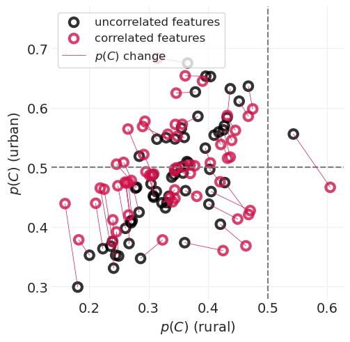
包括特征相关性#
点移动是因为跨特征的信息传递提供了更好的 \(p(C)\) 估计
农村地区与城市地区避孕药具使用率差异之间存在负相关关系
当一个地区的农村地区避孕药具使用率很高时,差异会更小(即城市地区也将具有较高的避孕药具使用率)
当农村地区避孕药具使用率较低时,城市地区将更加不同(即城市地区仍然倾向于具有较高的避孕药具使用率)
奖励:非居中(又名变换)先验#
不方便的后验#
由负对数似然中的陡峭曲率引起的不高效 MCMC
哈密顿蒙特卡洛在探索陡峭表面时遇到困难
导致“发散”跃迁
“冲破滑板公园的墙壁”
当哈密顿量在提议的开始/结束之间发生剧烈变化时检测到
变换先验以使其成为“更平滑的滑板公园”有所帮助
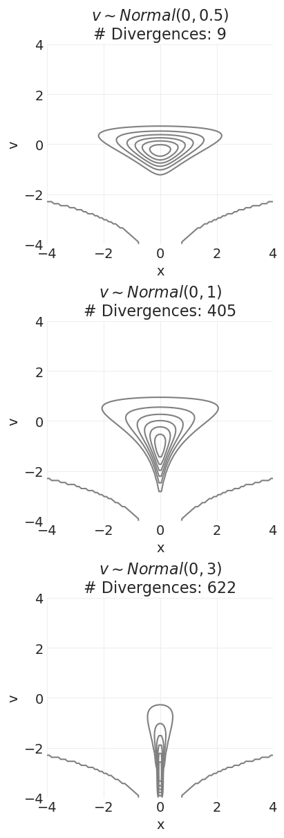
示例:魔鬼漏斗先验#
随着 \(\sigma_v\) 的增加,先验概率表面中会形成一个讨厌的槽,哈密顿动力学很难对其进行采样——即,滑板公园太陡峭和狭窄。
我太懒了,无法编写 McElreath 用来可视化每个发散路径的精美 HMC 动画。但是,我们仍然可以验证,当我们在魔鬼漏斗先验中增加 v 先验的 \(\sigma\) 时,发散的数量会增加。
居中先验模型#
from functools import partial

xs = vs = np.linspace(-4, 4, 100)


def prior_devils_funnel(xs, vs, sigma_v=0.5):

    log_prior_v = stats.norm(0, sigma_v).logpdf(vs)
    log_prior_x = stats.norm(0, np.exp(vs)).logpdf(xs)

    log_prior = log_prior_v + log_prior_x
    return np.exp(log_prior - log_prior.max())


# Loop over sigma_v, and show that divergences increase
# as the depth and narrowness of the trough increases
# for low values of v
sigma_vs = [0.5, 1, 3]
n_sigma_vs = len(sigma_vs)
fig, axs = plt.subplots(3, 1, figsize=(4, 4 * n_sigma_vs))

for ii, sigma_v in enumerate(sigma_vs):
    with pm.Model() as centered_devils_funnel:
        v = pm.Normal("v", 0, sigma_v)
        x = pm.Normal("x", 0, pm.math.exp(v))
        centered_devils_funnel_inference = pm.sample()
        n_divergences = centered_devils_funnel_inference.sample_stats.diverging.sum().values

    prior = partial(prior_devils_funnel, sigma_v=sigma_v)
    plt.sca(axs[ii])
    utils.plot_2d_function(xs, ys, prior, colors="gray", ax=axs[ii])
    plt.xlabel("x")
    plt.ylabel("v")
    plt.title(f"$v \sim Normal(0, {sigma_v})$\n# Divergences: {n_divergences}")
Initializing NUTS using jitter+adapt_diag...
Multiprocess sampling (4 chains in 4 jobs)
NUTS: [v, x]
Sampling 4 chains for 1_000 tune and 1_000 draw iterations (4_000 + 4_000 draws total) took 1 seconds.
There were 9 divergences after tuning. Increase `target_accept` or reparameterize.
Initializing NUTS using jitter+adapt_diag...
Multiprocess sampling (4 chains in 4 jobs)
NUTS: [v, x]
Sampling 4 chains for 1_000 tune and 1_000 draw iterations (4_000 + 4_000 draws total) took 1 seconds.
There were 405 divergences after tuning. Increase `target_accept` or reparameterize.
The rhat statistic is larger than 1.01 for some parameters. This indicates problems during sampling. See https://arxiv.org/abs/1903.08008 for details
The effective sample size per chain is smaller than 100 for some parameters.  A higher number is needed for reliable rhat and ess computation. See https://arxiv.org/abs/1903.08008 for details
Initializing NUTS using jitter+adapt_diag...
Multiprocess sampling (4 chains in 4 jobs)
NUTS: [v, x]
Sampling 4 chains for 1_000 tune and 1_000 draw iterations (4_000 + 4_000 draws total) took 1 seconds.
There were 622 divergences after tuning. Increase `target_accept` or reparameterize.
The rhat statistic is larger than 1.01 for some parameters. This indicates problems during sampling. See https://arxiv.org/abs/1903.08008 for details
The effective sample size per chain is smaller than 100 for some parameters.  A higher number is needed for reliable rhat and ess computation. See https://arxiv.org/abs/1903.08008 for details
怎么办?#
更小的步长:更好地处理陡峭度,但需要更长的时间来探索后验
重新参数化(变换)以使表面更平滑
非居中先验#
我们添加一个辅助变量 \(z\),它具有平滑的概率表面。然后我们对该辅助变量进行采样,并对其进行变换以获得目标变量分布。对于魔鬼漏斗先验的情况
sigma_vs = [0.5, 1, 3]
n_sigma_vs = len(sigma_vs)
fig, axs = plt.subplots(3, 1, figsize=(4, 4 * n_sigma_vs))


def prior_noncentered_devils_funnel(xs, vs, sigma_v=0.5):
    """Reparamterize into a smoother auxilary variable space"""
    log_prior_v = stats.norm(0, sigma_v).logpdf(vs)
    log_prior_z = stats.norm(0, 1).logpdf(xs)
    log_prior = log_prior_v + log_prior_z
    return np.exp(log_prior - log_prior.max())


for ii, sigma_v in enumerate(sigma_vs):
    with pm.Model() as noncentered_devils_funnel:
        v = pm.Normal("v", 0, sigma_v)
        z = pm.Normal("z", 0, 1)
        # Record x for reporting
        x = pm.Deterministic("x", z * pm.math.exp(v))
        noncentered_devils_funnel_inference = pm.sample()
        n_divergences = noncentered_devils_funnel_inference.sample_stats.diverging.sum().values

    prior = partial(prior_noncentered_devils_funnel, sigma_v=sigma_v)
    plt.sca(axs[ii])
    utils.plot_2d_function(xs, ys, prior, colors="gray", ax=axs[ii])
    plt.xlabel("z")
    plt.ylabel("v")
    plt.title(f"$v \sim$ Normal(0, {sigma_v})\n# Divergences: {n_divergences}")
Initializing NUTS using jitter+adapt_diag...
Multiprocess sampling (4 chains in 4 jobs)
NUTS: [v, z]
Sampling 4 chains for 1_000 tune and 1_000 draw iterations (4_000 + 4_000 draws total) took 1 seconds.
Initializing NUTS using jitter+adapt_diag...
Multiprocess sampling (4 chains in 4 jobs)
NUTS: [v, z]
Sampling 4 chains for 1_000 tune and 1_000 draw iterations (4_000 + 4_000 draws total) took 1 seconds.
Initializing NUTS using jitter+adapt_diag...
Multiprocess sampling (4 chains in 4 jobs)
NUTS: [v, z]
Sampling 4 chains for 1_000 tune and 1_000 draw iterations (4_000 + 4_000 draws total) took 1 seconds.
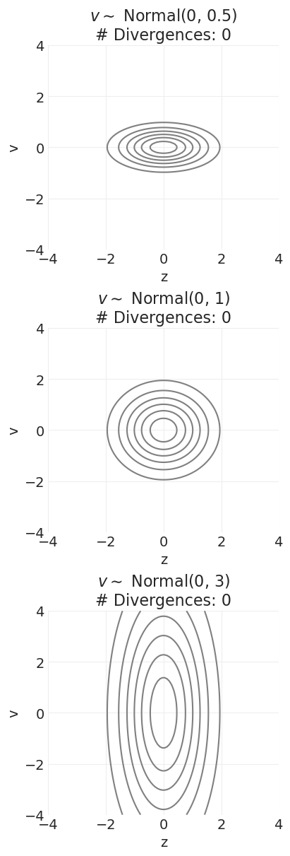
通过重新参数化,我们可以对多维正态分布进行采样,这些分布在对数空间中是更平滑的抛物线。
我们可以看到,对于所有先验方差值,发散的数量都持续减少。
检查 HMC 诊断#
az.summary(noncentered_devils_funnel_inference)["r_hat"]
v    1.0
x    1.0
z    1.0
Name: r_hat, dtype: float64
az.plot_trace(noncentered_devils_funnel_inference);
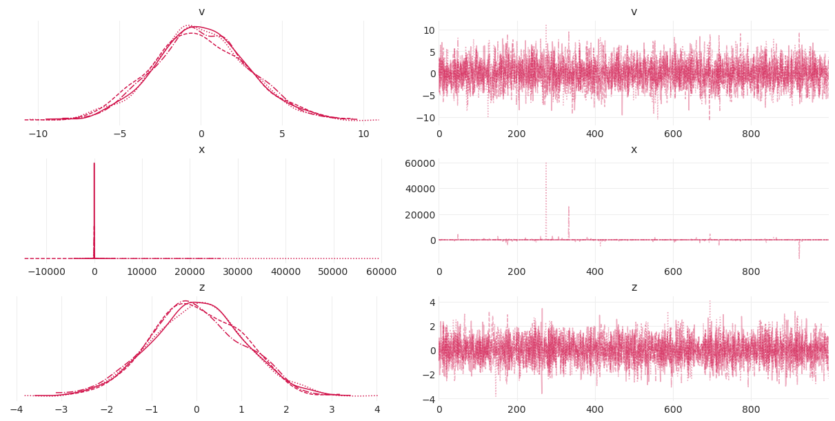
诊断看起来不错 👍
Rhats = 1\(v\) 和 \(z\) 链表现出“模糊毛毛虫”行为
Cholesky 因子和相关矩阵#
Cholesky 因子 \(\bf L\) 提供了一种有效的方法来编码相关矩阵 \(\Omega\)(比完整的相关矩阵需要更少的浮点数)
\(\Omega = \bf LL^T\)
\(\bf L\) 是一个下三角矩阵
我们可以使用 \(\Omega\) 的 Cholesky 分解 \(\bf L\) 对具有相关性 \(\Omega\) 和标准差 \(\sigma_i\) 的数据进行采样,如下所示
其中 \(\bf Z\) 是从标准正态分布中采样的 z 分数矩阵
演示从 Cholesky 因子重建相关矩阵#
orig_corr = np.array([[1, 0.6], [0.6, 1]])
print("Ground-truth Correlation Matrix\n", orig_corr)

L = np.linalg.cholesky(orig_corr)
print("\nCholesky Matrix of correlation matrix, L\n", L)
print("\nReconstructed correlation matrix from L\n", L @ L.T)
Ground-truth Correlation Matrix
 [[1.  0.6]
 [0.6 1. ]]

Cholesky Matrix of correlation matrix, L
 [[1.  0. ]
 [0.6 0.8]]

Reconstructed correlation matrix from L
 [[1.  0.6]
 [0.6 1. ]]
演示从 z 分数和 Cholesky 因子采样随机相关矩阵#
np.random.seed(12345)
N = 100_000
orig_sigmas = [2, 0.5]

# Matrix of z-score samples
Z = stats.norm().rvs(size=(2, N))
print("Raw z-score samples are indpendent\n", np.corrcoef(Z[0], Z[1]))

# Transform Z-scores using the Cholesky factorization of the correlation matrix
sLZ = np.diag(orig_sigmas) @ L @ Z

corr_sLZ = np.corrcoef(sLZ[0], sLZ[1])
print("\nCholesky-transformed z-scores have original correlation encoded\n", corr_sLZ)
assert np.isclose(orig_corr[0, 1], corr_sLZ[0, 1], atol=0.01)

std_sLZ = sLZ.std(axis=1)
print("\nOriginal std devs also encoded in transformed z-scores:\n", std_sLZ)
assert np.isclose(orig_sigmas[0], std_sLZ[0], atol=0.01)
assert np.isclose(orig_sigmas[1], std_sLZ[1], atol=0.01)
Raw z-score samples are indpendent
 [[1.         0.00293945]
 [0.00293945 1.        ]]

Cholesky-transformed z-scores have original correlation encoded
 [[1.         0.60268456]
 [0.60268456 1.        ]]

Original std devs also encoded in transformed z-scores:
 [2.00212936 0.50024976]
何时使用变换先验#
取决于上下文
居中
每个聚类/子组中的大量数据
似然主导场景
非居中
许多聚类/子组,其中一些聚类中的数据稀疏
先验主导场景
许可证声明#
此示例库中的所有笔记本均根据 MIT 许可证 提供,该许可证允许修改和再分发用于任何用途,前提是保留版权和许可证声明。
引用 PyMC 示例#
要引用此笔记本,请使用 Zenodo 为 pymc-examples 存储库提供的 DOI。
重要提示
许多笔记本都改编自其他来源:博客、书籍……在这种情况下,您也应该引用原始来源。
另请记住引用您的代码使用的相关库。
这是一个 bibtex 中的引用模板
@incollection{citekey,
  author    = "<notebook authors, see above>",
  title     = "<notebook title>",
  editor    = "PyMC Team",
  booktitle = "PyMC examples",
  doi       = "10.5281/zenodo.5654871"
}
一旦呈现,它可能看起来像