


是什么驱动了分享?#
Koster & Leckie (2014) Arang Dak 数据集#
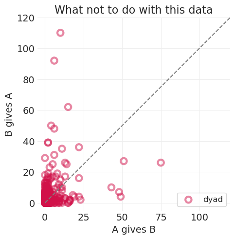
25 个家庭之间食物转移的年份
300 个 dyad,即 \(\binom{25}{2} = 300\)
2871 个食物转移(“礼物”)观察值
科学问题:估计量#
有多少分享可以用互惠性解释?
有多少可以用广义给予解释?
SHARING = utils.load_data("KosterLeckie")
SHARING.head()
| hidA | hidB | did | giftsAB | giftsBA | offset | drel1 | drel2 | drel3 | drel4 | dlndist | dass | d0125 | |
|---|---|---|---|---|---|---|---|---|---|---|---|---|---|
| 0 | 1 | 2 | 1 | 0 | 4 | 0.000 | 0 | 0 | 1 | 0 | -2.790 | 0.000 | 0 |
| 1 | 1 | 3 | 2 | 6 | 31 | -0.003 | 0 | 1 | 0 | 0 | -2.817 | 0.044 | 0 |
| 2 | 1 | 4 | 3 | 2 | 5 | -0.019 | 0 | 1 | 0 | 0 | -1.886 | 0.025 | 0 |
| 3 | 1 | 5 | 4 | 4 | 2 | 0.000 | 0 | 1 | 0 | 0 | -1.892 | 0.011 | 0 |
| 4 | 1 | 6 | 5 | 8 | 2 | -0.003 | 1 | 0 | 0 | 0 | -3.499 | 0.022 | 0 |
utils.plot_scatter(SHARING.giftsAB, SHARING.giftsBA, color="C0", label="dyad", alpha=0.5)
plt.plot((0, 120), (0, 120), linestyle="--", color="gray")
plt.axis("square")
plt.xlabel("A gives B")
plt.ylabel("B gives A")
plt.xlim([-5, 120])
plt.ylim([-5, 120])
plt.title("What not to do with this data")
plt.legend();
使用因果图改进分析#
utils.draw_causal_graph(
    edge_list=[
        ("H_A", "G_AB"),
        ("H_B", "G_AB"),
        ("H_A", "T_AB"),
        ("H_B", "T_AB"),
        ("H_A", "T_BA"),
        ("H_B", "T_BA"),
        ("T_AB", "G_AB"),
        ("T_BA", "G_AB"),
    ],
    node_props={
        "H_A": {"label": "household A, H_A"},
        "H_B": {"label": "household B, H_B"},
        "G_AB": {"label": "A gives to B, G_AB"},
        "T_AB": {"label": "Social tie from A to B, T_AB", "style": "dashed"},
        "T_BA": {"label": "Social tie from B to A, T_BA", "style": "dashed"},
        "unobserved": {"style": "dashed"},
    },
)

1) 估计量#
从简单开始,暂时忽略家庭效应#
utils.draw_causal_graph(
    edge_list=[
        ("H_A", "G_AB"),
        ("H_B", "G_AB"),
        ("H_A", "T_AB"),
        ("H_B", "T_AB"),
        ("H_A", "T_BA"),
        ("H_B", "T_BA"),
        ("T_AB", "G_AB"),
        ("T_BA", "G_AB"),
    ],
    node_props={
        "H_A": {"color": "blue"},
        "H_B": {"color": "blue"},
        "T_AB": {"style": "dashed", "color": "red"},
        "T_BA": {"style": "dashed", "color": "red"},
        "unobserved": {"style": "dashed"},
    },
    edge_props={
        ("T_AB", "G_AB"): {"color": "red"},
        ("T_BA", "G_AB"): {"color": "red"},
        ("H_A", "G_AB"): {"color": "blue"},
        ("H_B", "G_AB"): {"color": "blue", "label": " backdoor\npaths", "fontcolor": "blue"},
        ("H_A", "T_AB"): {"color": "blue"},
        ("H_A", "T_BA"): {"color": "blue"},
        ("H_B", "T_AB"): {"color": "blue"},
        ("H_B", "T_BA"): {"color": "blue"},
    },
)

首先,我们将忽略后门路径以获得良好的流程,并使模型运行起来,然后再添加它们
2) 生成模型#
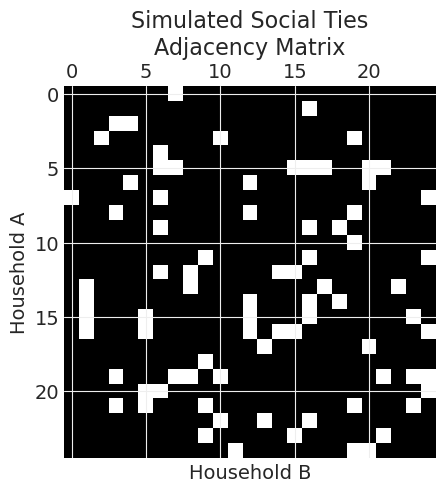
模拟社交网络#
from itertools import combinations

np.random.seed(123)

N = 25
dyads = list(combinations(np.arange(N), 2))

# convert to numpy for np.where
DYADS = np.array(dyads)
N_DYADS = len(DYADS)

print(f"N dyads: {N_DYADS}")
print(dyads[:91])

# Simulate "friendship", in which ties are shared
P_FRIENDSHIP = 0.1
FRIENDSHIP = stats.bernoulli(p=P_FRIENDSHIP).rvs(size=N_DYADS)

# Simulate directed ties. Note: there can be ties that are not reciprocal
ALPHA = -3.0  # base rate has low probability
BASE_TIE_PROBABILITY = utils.invlogit(ALPHA)
print(f"\nBase non-friend social tie probability: {BASE_TIE_PROBABILITY:.2}")


def get_dyad_index(source, target):
    # dyads are symmetric, but ordered by definition,
    # so ensure valid lookup by sorting
    ii, jj = sorted([source, target])
    return np.where((DYADS[:, 0] == ii) & (DYADS[:, 1] == jj))[0][0]


# Simulate gift-giving
TIES = np.zeros((N, N)).astype(int)
for source in range(N):
    for target in range(N):
        if source != target:
            dyad_index = get_dyad_index(source, target)
            # Sample directed edge -- friends always share ties,
            # but there's also a base rate of sharing ties w/o friendship
            is_friend = FRIENDSHIP[dyad_index]
            p_tie = is_friend + (1 - is_friend) * BASE_TIE_PROBABILITY
            TIES[source, target] = stats.bernoulli(p_tie).rvs()
N dyads: 300
[(0, 1), (0, 2), (0, 3), (0, 4), (0, 5), (0, 6), (0, 7), (0, 8), (0, 9), (0, 10), (0, 11), (0, 12), (0, 13), (0, 14), (0, 15), (0, 16), (0, 17), (0, 18), (0, 19), (0, 20), (0, 21), (0, 22), (0, 23), (0, 24), (1, 2), (1, 3), (1, 4), (1, 5), (1, 6), (1, 7), (1, 8), (1, 9), (1, 10), (1, 11), (1, 12), (1, 13), (1, 14), (1, 15), (1, 16), (1, 17), (1, 18), (1, 19), (1, 20), (1, 21), (1, 22), (1, 23), (1, 24), (2, 3), (2, 4), (2, 5), (2, 6), (2, 7), (2, 8), (2, 9), (2, 10), (2, 11), (2, 12), (2, 13), (2, 14), (2, 15), (2, 16), (2, 17), (2, 18), (2, 19), (2, 20), (2, 21), (2, 22), (2, 23), (2, 24), (3, 4), (3, 5), (3, 6), (3, 7), (3, 8), (3, 9), (3, 10), (3, 11), (3, 12), (3, 13), (3, 14), (3, 15), (3, 16), (3, 17), (3, 18), (3, 19), (3, 20), (3, 21), (3, 22), (3, 23), (3, 24), (4, 5)]

Base non-friend social tie probability: 0.047
plt.matshow(TIES, cmap="gray")
plt.ylabel("Household A")
plt.xlabel("Household B")
plt.title("Simulated Social Ties\nAdjacency Matrix");
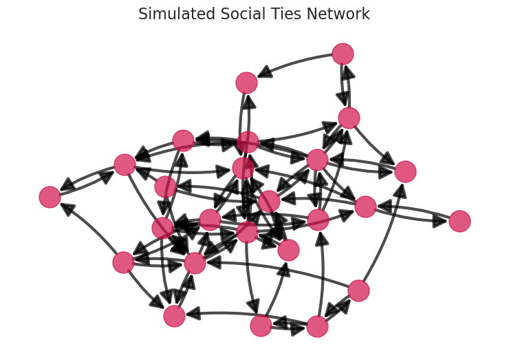
import networkx as nx

TIES_LAYOUT_POSITION = utils.plot_graph(TIES)
plt.title("Simulated Social Ties Network");
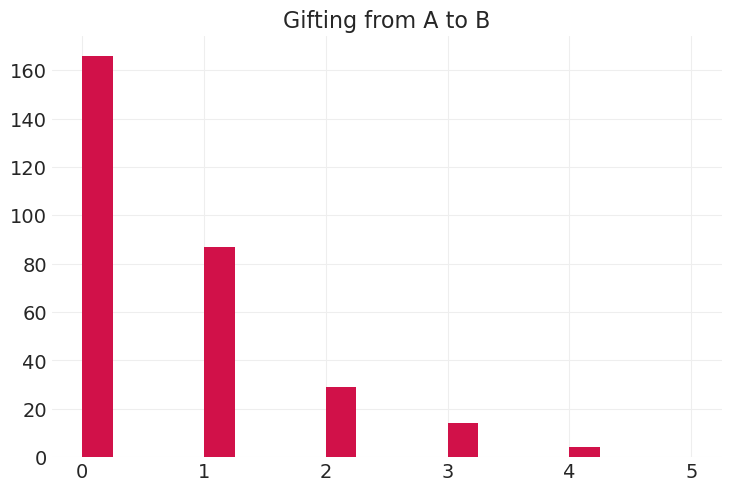
从社交网络模拟送礼行为#
giftsAB = np.zeros(N_DYADS)
giftsBA = np.zeros(N_DYADS)
lam = np.log([0.5, 2])

for ii, (A, B) in enumerate(DYADS):
    lambdaAB = np.exp(lam[TIES[A, B]])
    giftsAB[ii] = stats.poisson(mu=lambdaAB).rvs()

    lambdaBA = np.exp(lam[TIES[B, A]])
    giftsBA[ii] = stats.poisson(mu=lambdaBA).rvs()

## Put simulation into a dataframe for fitting function
simulated_gifts = pd.DataFrame(
    {
        "giftsAB": giftsAB.astype(int),
        "giftsBA": giftsBA.astype(int),
        "did": np.arange(N_DYADS).astype(int),
    }
)

simulated_gifts
| giftsAB | giftsBA | did | |
|---|---|---|---|
| 0 | 1 | 0 | 0 |
| 1 | 0 | 1 | 1 |
| 2 | 2 | 0 | 2 |
| 3 | 0 | 1 | 3 |
| 4 | 0 | 0 | 4 |
| ... | ... | ... | ... |
| 295 | 0 | 1 | 295 |
| 296 | 0 | 0 | 296 |
| 297 | 1 | 0 | 297 |
| 298 | 0 | 0 | 298 |
| 299 | 0 | 0 | 299 |
300 行 × 3 列
3) 统计模型#
似然函数#
全局送礼先验#
后验关系#
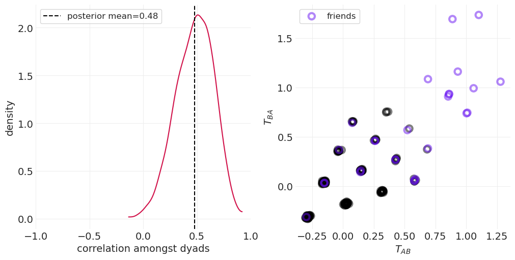
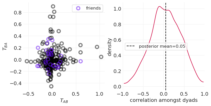
def plot_posterior_reciprocity(inference, ax=None):
az.plot_dist(inference.posterior["corrcoef_T"], ax=ax)
posterior_mean = inference.posterior["corrcoef_T"].mean().values
plt.axvline(
posterior_mean, label=f"posterior mean={posterior_mean:0.2f}", color="k", linestyle="--"
)
plt.xlim([-1, 1])
plt.xlabel("correlation amongst dyads")
plt.ylabel("density")
plt.legend()
def plot_posterior_household_ties(inference, color_friends=False, ax=None):
T = inference.posterior.mean(dim=("chain", "draw"))["T"]
T_AB = T[:, 0]
T_BA = T[:, 1]
if color_friends:
colors = ["black", "C4"]
labels = [None, "friends"]
for is_friends in [0, 1]:
mask = FRIENDSHIP == is_friends
utils.plot_scatter(
T_AB[mask],
T_BA[mask],
color=colors[is_friends],
alpha=0.5,
label=labels[is_friends],
)
else:
utils.plot_scatter(T_AB, T_BA, color="C0", label="dyadic ties")
plt.xlabel("$T_{AB}$")
plt.ylabel("$T_{BA}$")
plt.legend();
_, axs = plt.subplots(1, 2, figsize=(10, 5))
plt.sca(axs[0])
plot_posterior_reciprocity(simulated_social_ties_inference, ax=axs[0])
plt.sca(axs[1])
plot_posterior_household_ties(simulated_social_ties_inference, color_friends=True, ax=axs[1])
4) 分析数据#
在真实数据样本上运行模型
social_ties_model, social_ties_inference = fit_social_ties_model(SHARING)
Initializing NUTS using jitter+adapt_diag...
Multiprocess sampling (4 chains in 4 jobs)
NUTS: [alpha, rho, z]
Sampling 4 chains for 1_000 tune and 1_000 draw iterations (4_000 + 4_000 draws total) took 11 seconds.
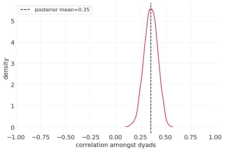
后验相关性#
az.summary(social_ties_inference, var_names="rho_corr")
| 均值 | 标准差 | hdi_3% | hdi_97% | mcse_mean | mcse_sd | ess_bulk | ess_tail | r_hat | |
|---|---|---|---|---|---|---|---|---|---|
| rho_corr[0, 0] | 1.000 | 0.000 | 1.000 | 1.000 | 0.000 | 0.000 | 4000.0 | 4000.0 | NaN |
| rho_corr[0, 1] | 0.352 | 0.068 | 0.231 | 0.479 | 0.003 | 0.002 | 539.0 | 1272.0 | 1.01 |
| rho_corr[1, 0] | 0.352 | 0.068 | 0.231 | 0.479 | 0.003 | 0.002 | 539.0 | 1272.0 | 1.01 |
| rho_corr[1, 1] | 1.000 | 0.000 | 1.000 | 1.000 | 0.000 | 0.000 | 4089.0 | 3939.0 | 1.00 |
plot_posterior_reciprocity(social_ties_inference)
引入家庭给予/接受混淆因素#
2) 生成模型#
模拟包括未测量的家庭财富#
我们使用相同的社会关系网络,但根据(未测量的)家庭财富来增加送礼行为
较富裕的家庭给予更多
较贫穷的家庭接受更多
np.random.seed(123)
giftsAB = np.zeros(N_DYADS)
giftsBA = np.zeros(N_DYADS)

LAMBDA = np.log([0.5, 2])
BETA_WG = 0.5  #  Effect of (standardized) household wealth on giving -> the wealthy give more
BETA_WR = -1  # Effect of household wealth on receiving -> weathy recieve less

WEALTH = stats.norm.rvs(size=N)  # standardized wealth

for ii, (A, B) in enumerate(DYADS):
    lambdaAB = np.exp(LAMBDA[TIES[A, B]] + BETA_WG * WEALTH[A] + BETA_WR * WEALTH[B])
    giftsAB[ii] = stats.poisson(mu=lambdaAB).rvs()

    lambdaBA = np.exp(LAMBDA[TIES[B, A]] + BETA_WG * WEALTH[B] + BETA_WR * WEALTH[A])
    giftsBA[ii] = stats.poisson(mu=lambdaBA).rvs()

## Put simulation into a dataframe for fitting function
simulated_wealth_gifts = pd.DataFrame(
    {
        "giftsAB": giftsAB.astype(int),
        "giftsBA": giftsBA.astype(int),
        "hidA": DYADS[:, 0],
        "hidB": DYADS[:, 1],
        "did": np.arange(N_DYADS).astype(int),
    }
)

simulated_wealth_gifts
| giftsAB | giftsBA | hidA | hidB | did | |
|---|---|---|---|---|---|
| 0 | 0 | 1 | 0 | 1 | 0 |
| 1 | 0 | 2 | 0 | 2 | 1 |
| 2 | 1 | 2 | 0 | 3 | 2 |
| 3 | 1 | 0 | 0 | 4 | 3 |
| 4 | 0 | 5 | 0 | 5 | 4 |
| ... | ... | ... | ... | ... | ... |
| 295 | 1 | 3 | 21 | 23 | 295 |
| 296 | 5 | 0 | 21 | 24 | 296 |
| 297 | 0 | 2 | 22 | 23 | 297 |
| 298 | 0 | 3 | 22 | 24 | 298 |
| 299 | 3 | 0 | 23 | 24 | 299 |
300 行 × 5 列
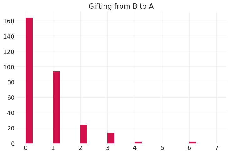
# plt.hist(simulated_wealth_gifts.giftsAB, bins=simulated_gifts.giftsAB.max(), width=.25);
# plt.title("Gifting from A to B\n(including household wealth)");
# plt.hist(simulated_wealth_gifts.giftsBA, bins=simulated_gifts.giftsBA.max(), width=.25);
# plt.title("Gifting from B to A\n(including household wealth)");
3) 统计模型#
\(G_{A,B}\) - 家庭 \(A,B\) 的广义给予
\(R_{A,B}\) - 家庭 \(A,B\) 的广义接受
使用 \(\text{MVNormal}\) 对给予和接受协方差进行建模
似然函数#
全局送礼先验#
相关社会关系先验#
在模拟数据上拟合财富送礼模型(验证)#
def fit_giving_receiving_model(data, eta=2):
    n_dyads = len(data)
    n_correlated_features = 2

    dyad_id = data.did.values.astype(int)
    household_A_id = data.hidA.values.astype(int)
    household_B_id = data.hidB.values.astype(int)

    # Data are 1-indexed
    if np.min(dyad_id) == 1:
        dyad_id -= 1
        household_A_id -= 1
        household_B_id -= 1

    n_households = np.max([household_A_id, household_B_id]) + 1

    with pm.Model() as model:

        # single, global alpha
        alpha = pm.Normal("alpha", 0, 1)

        # Social ties interaction; shared sigma
        sigma_T = pm.Exponential.dist(1)
        chol_T, corr_T, std_T = pm.LKJCholeskyCov(
            "rho_T", eta=eta, n=n_correlated_features, sd_dist=sigma_T
        )
        z_T = pm.Normal("z_T", 0, 1, shape=(n_dyads, n_correlated_features))
        T = pm.Deterministic("T", chol_T.dot(z_T.T).T)

        # Giving-receiving interaction; full covariance
        sigma_GR = pm.Exponential.dist(1, shape=n_correlated_features)
        chol_GR, corr_GR, std_GR = pm.LKJCholeskyCov(
            "rho_GR", eta=eta, n=n_correlated_features, sd_dist=sigma_GR
        )
        z_GR = pm.Normal("z_GR", 0, 1, shape=(n_households, n_correlated_features))
        GR = pm.Deterministic("GR", chol_GR.dot(z_GR.T).T)

        lambda_AB = pm.Deterministic(
            "lambda_AB",
            pm.math.exp(alpha + T[dyad_id, 0] + GR[household_A_id, 0] + GR[household_B_id, 1]),
        )
        lambda_BA = pm.Deterministic(
            "lambda_BA",
            pm.math.exp(alpha + T[dyad_id, 1] + GR[household_B_id, 0] + GR[household_A_id, 1]),
        )

        # Record quantities for reporting
        pm.Deterministic("corrcoef_T", corr_T[0, 1])
        pm.Deterministic("std_T", std_T)

        pm.Deterministic("corrcoef_GR", corr_GR[0, 1])
        pm.Deterministic("std_GR", std_GR)

        G_AB = pm.Poisson("G_AB", lambda_AB, observed=data.giftsAB)
        G_BA = pm.Poisson("G_BA", lambda_BA, observed=data.giftsBA)

        inference = pm.sample(target_accept=0.9)
        inference = pm.compute_log_likelihood(inference, extend_inferencedata=True)
    return model, inference
simulated_gr_model, simulated_gr_inference = fit_giving_receiving_model(simulated_wealth_gifts)
Initializing NUTS using jitter+adapt_diag...
Multiprocess sampling (4 chains in 4 jobs)
NUTS: [alpha, rho_T, z_T, rho_GR, z_GR]
Sampling 4 chains for 1_000 tune and 1_000 draw iterations (4_000 + 4_000 draws total) took 26 seconds.
The rhat statistic is larger than 1.01 for some parameters. This indicates problems during sampling. See https://arxiv.org/abs/1903.08008 for details
The effective sample size per chain is smaller than 100 for some parameters.  A higher number is needed for reliable rhat and ess computation. See https://arxiv.org/abs/1903.08008 for details
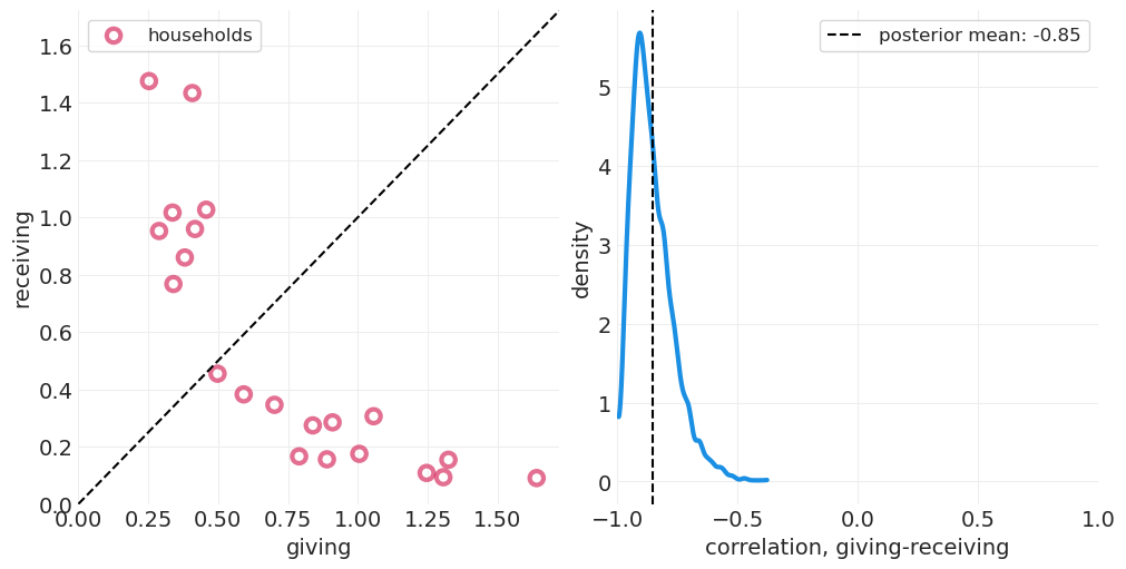
az.summary(simulated_gr_inference, var_names=["corrcoef_T", "corrcoef_GR"])
| 均值 | 标准差 | hdi_3% | hdi_97% | mcse_mean | mcse_sd | ess_bulk | ess_tail | r_hat | |
|---|---|---|---|---|---|---|---|---|---|
| corrcoef_T | 0.467 | 0.258 | -0.008 | 0.921 | 0.016 | 0.011 | 260.0 | 579.0 | 1.02 |
| corrcoef_GR | -0.853 | 0.087 | -0.981 | -0.694 | 0.003 | 0.002 | 989.0 | 1727.0 | 1.00 |
def plot_wealth_gifting_posterior(inference, data_range=None):
    posterior_alpha = inference.posterior["alpha"]
    posterior_GR = inference.posterior["GR"]

    log_posterior_giving = posterior_alpha + posterior_GR[:, :, :, 0]  # Household A
    log_posterior_receiving = posterior_alpha + posterior_GR[:, :, :, 1]  # Household B

    posterior_receiving = np.exp(log_posterior_giving.mean(dim=("chain", "draw")))
    posterior_giving = np.exp(log_posterior_receiving.mean(dim=("chain", "draw")))

    # Household giving/receiving
    _, axs = plt.subplots(1, 2, figsize=(10, 5))
    plt.sca(axs[0])
    utils.plot_scatter(posterior_receiving, posterior_giving, color="C0", label="households")
    if data_range is None:
        axis_max = np.max(posterior_receiving.values.ravel()) * 1.05
        data_range = (0, axis_max)
    plt.xlabel("giving")
    plt.ylabel("receiving")
    plt.legend()
    plt.plot(data_range, data_range, color="k", linestyle="--")
    plt.xlim(data_range)
    plt.ylim(data_range)

    # Giving/receiving correlation distribution
    plt.sca(axs[1])
    az.plot_dist(inference.posterior["corrcoef_GR"], color="C1", plot_kwargs={"linewidth": 3})
    cc_mean = inference.posterior["corrcoef_GR"].mean()
    plt.axvline(cc_mean, color="k", linestyle="--", label=f"posterior mean: {cc_mean:1.2}")
    plt.xlim([-1, 1])
    plt.legend()
    plt.ylabel("density")
    plt.xlabel("correlation, giving-receiving")


def plot_dyadic_ties(inference):
    inference = wealth_gifts_inference
    T = inference.posterior.mean(dim=("chain", "draw"))["T"]
    utils.plot_scatter(T[:, 0], T[:, 1], color="C0", label="dyadic ties")
    plt.xlabel("Household A")
    plt.ylabel("Household B")
    plt.legend()
plot_wealth_gifting_posterior(simulated_gr_inference)
_, axs = plt.subplots(1, 2, figsize=(8, 4))
plt.sca(axs[0])
plot_posterior_household_ties(simulated_gr_inference, color_friends=True)

plt.sca(axs[1])
plot_posterior_reciprocity(simulated_gr_inference)
在真实数据上拟合#
gr_model, gr_inference = fit_giving_receiving_model(SHARING)
Initializing NUTS using jitter+adapt_diag...
Multiprocess sampling (4 chains in 4 jobs)
NUTS: [alpha, rho_T, z_T, rho_GR, z_GR]
Sampling 4 chains for 1_000 tune and 1_000 draw iterations (4_000 + 4_000 draws total) took 26 seconds.
az.summary(gr_inference, var_names=["corrcoef_T", "corrcoef_GR"])
| 均值 | 标准差 | hdi_3% | hdi_97% | mcse_mean | mcse_sd | ess_bulk | ess_tail | r_hat | |
|---|---|---|---|---|---|---|---|---|---|
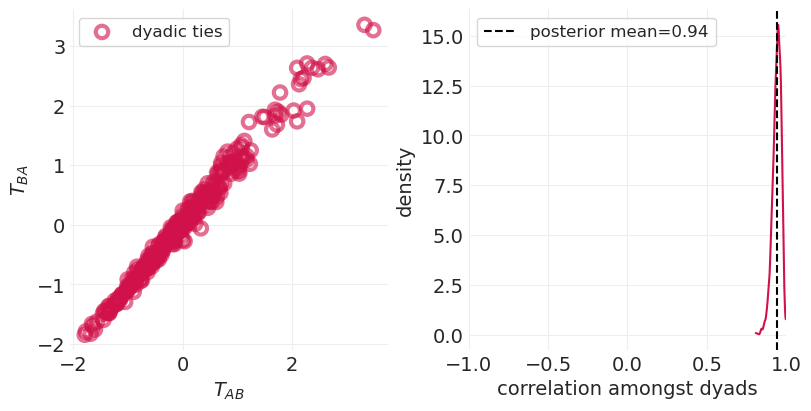
| corrcoef_T | 0.941 | 0.027 | 0.893 | 0.988 | 0.001 | 0.001 | 767.0 | 1300.0 | 1.0 |
| corrcoef_GR | -0.529 | 0.213 | -0.892 | -0.126 | 0.006 | 0.004 | 1327.0 | 1819.0 | 1.0 |
plot_wealth_gifting_posterior(gr_inference)
_, axs = plt.subplots(1, 2, figsize=(8, 4))
plt.sca(axs[0])
plot_posterior_household_ties(gr_inference)
plt.sca(axs[1])
plot_posterior_reciprocity(gr_inference)
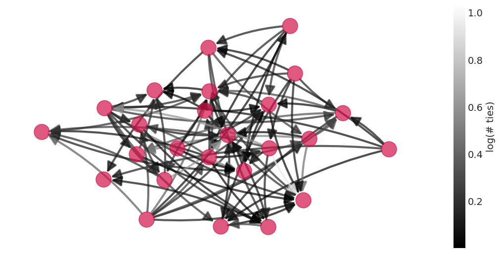
绘制后验均值社交图#
def plot_posterior_mean_graph(
    inference, rescale_probs=False, edge_colormap="gray", title=None, **plot_graph_kwargs
):
    """Plot the simulated ties graph, weighting each tie connection's edge color by
    a model's posterior mean probability of T_AB.
    """
    T = inference.posterior["T"]
    mean_lambda_ties = np.exp(T.mean(dim=("chain", "draw"))[:, 0])
    _, axs = plt.subplots(1, 2, figsize=(10, 5), width_ratios=[20, 1])

    plt.sca(axs[0])
    plt.set_cmap(edge_colormap)
    A, B = np.nonzero(TIES)

    G = nx.DiGraph()
    edge_color = []
    for ii, (A, B) in enumerate(DYADS):
        ii, jj = sorted([A, B])
        dyad_idx = np.where((DYADS[:, 0] == A) & (DYADS[:, 1] == B))[0][0].astype(int)
        weight = mean_lambda_ties[dyad_idx]

        # include edges that predict one or more social ties
        if weight >= 1:
            G.add_edge(A, B, weight=weight)
            edge_color.append(weight)

    edge_color = np.log(np.array(edge_color))
    utils.plot_graph(G, edge_color=edge_color, pos=TIES_LAYOUT_POSITION, **plot_graph_kwargs)
    plt.title(title)

    # Fake axis to hold colorbar
    plt.sca(axs[1])
    axs[1].set_aspect(0.0001)
    axs[1].set_visible(False)
    img = plt.imshow(np.array([[edge_color.min(), edge_color.max()]]))
    img.set_visible(False)

    clb = plt.colorbar(orientation="vertical", fraction=0.8, pad=0.1)
    clb.set_label("log(# ties)", rotation=90)
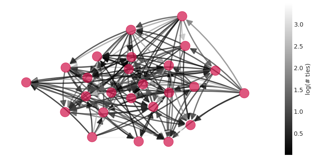
来自送礼模型的后验均值社交网络#
plot_posterior_mean_graph(social_ties_inference)
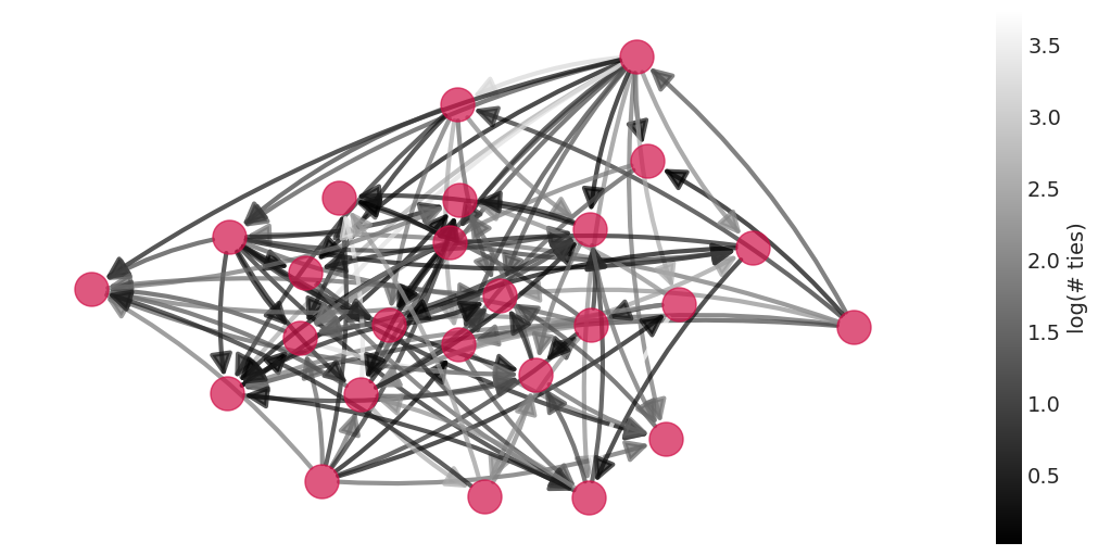
也纳入财富的模型的后验均值社交网络#
plot_posterior_mean_graph(gr_inference)
包括预测性家庭特征#
现在我们将预测特征添加到模型中。具体来说,我们将为以下内容添加 GLM 参数
每个 dyad 的关联特征 \(A_{AB}\) (例如,友谊), \(\beta_A\)。
家庭财富 \(W_{A,B}\) 对给予的影响, \(\beta_G\)
家庭财富 \(W_{A,B}\) 对接受的影响, \(\beta_R\)
似然函数#
全局先验#
相关社会关系先验#
相关给予/接受先验#
将观察到的混淆变量添加到模拟数据集#
# Add **observed** association feature
simulated_wealth_gifts.loc[:, "association"] = FRIENDSHIP

# Add **observed** wealth feature
simulated_wealth_gifts.loc[:, "wealthA"] = simulated_wealth_gifts.hidA.map(
    {ii: WEALTH[ii] for ii in range(N)}
)
simulated_wealth_gifts.loc[:, "wealthB"] = simulated_wealth_gifts.hidB.map(
    {ii: WEALTH[ii] for ii in range(N)}
)
def fit_giving_receiving_features_model(data, eta=2):
    n_dyads = len(data)
    n_correlated_features = 2

    dyad_id = data.did.values.astype(int)
    household_A_id = data.hidA.values.astype(int)
    household_B_id = data.hidB.values.astype(int)
    association_AB = data.association.values.astype(float)
    wealthA = data.wealthA.values.astype(float)
    wealthB = data.wealthB.values.astype(float)

    # Data are 1-indexed
    if np.min(dyad_id) == 1:
        dyad_id -= 1
        household_A_id -= 1
        household_B_id -= 1

    n_households = np.max([household_A_id, household_B_id]) + 1

    with pm.Model() as model:

        # Priors
        # single, global alpha
        alpha = pm.Normal("alpha", 0, 1)

        # global association and giving-receiving params
        beta_A = pm.Normal("beta_A", 0, 1)
        beta_G = pm.Normal("beta_G", 0, 1)
        beta_R = pm.Normal("beta_R", 0, 1)

        # Social ties interaction; shared sigma
        sigma_T = pm.Exponential.dist(1)
        chol_T, corr_T, std_T = pm.LKJCholeskyCov(
            "rho_T", eta=eta, n=n_correlated_features, sd_dist=sigma_T
        )
        z_T = pm.Normal("z_T", 0, 1, shape=(n_dyads, n_correlated_features))
        T = pm.Deterministic("T", chol_T.dot(z_T.T).T)

        T_AB = T[dyad_id, 0] + beta_A * association_AB
        T_BA = T[dyad_id, 1] + beta_A * association_AB

        # Giving-receiving interaction; full covariance
        sigma_GR = pm.Exponential.dist(1, shape=n_correlated_features)
        chol_GR, corr_GR, std_GR = pm.LKJCholeskyCov(
            "rho_GR", eta=eta, n=n_correlated_features, sd_dist=sigma_GR
        )
        z_GR = pm.Normal("z_GR", 0, 1, shape=(n_households, n_correlated_features))
        GR = pm.Deterministic("GR", chol_GR.dot(z_GR.T).T)

        G_A = GR[household_A_id, 0] + beta_G * wealthA
        G_B = GR[household_B_id, 0] + beta_G * wealthB

        R_A = GR[household_A_id, 1] + beta_R * wealthA
        R_B = GR[household_B_id, 1] + beta_R * wealthB

        lambda_AB = pm.Deterministic("lambda_AB", pm.math.exp(alpha + T_AB + G_A + R_B))
        lambda_BA = pm.Deterministic("lambda_BA", pm.math.exp(alpha + T_BA + G_B + R_A))

        # Record quantities for reporting
        pm.Deterministic("corrcoef_T", corr_T[0, 1])
        pm.Deterministic("std_T", std_T)

        pm.Deterministic("corrcoef_GR", corr_GR[0, 1])
        pm.Deterministic("std_GR", std_GR)
        pm.Deterministic("giving", beta_G)
        pm.Deterministic("receiving", beta_R)

        G_AB = pm.Poisson("G_AB", lambda_AB, observed=data.giftsAB)
        G_BA = pm.Poisson("G_BA", lambda_BA, observed=data.giftsBA)

        inference = pm.sample(target_accept=0.9)

        # Include log-likelihood for model comparison
        inference = pm.compute_log_likelihood(inference, extend_inferencedata=True)
    return model, inference
simulated_grf_model, simulated_grf_inference = fit_giving_receiving_features_model(
    simulated_wealth_gifts
)
Initializing NUTS using jitter+adapt_diag...
Multiprocess sampling (4 chains in 4 jobs)
NUTS: [alpha, beta_A, beta_G, beta_R, rho_T, z_T, rho_GR, z_GR]
Sampling 4 chains for 1_000 tune and 1_000 draw iterations (4_000 + 4_000 draws total) took 24 seconds.
The rhat statistic is larger than 1.01 for some parameters. This indicates problems during sampling. See https://arxiv.org/abs/1903.08008 for details
The effective sample size per chain is smaller than 100 for some parameters.  A higher number is needed for reliable rhat and ess computation. See https://arxiv.org/abs/1903.08008 for details
az.plot_dist(simulated_gr_inference.posterior["std_T"], color="C0", label="without Association")
az.plot_dist(simulated_grf_inference.posterior["std_T"], color="C1", label="with Association")
plt.xlabel("std T");
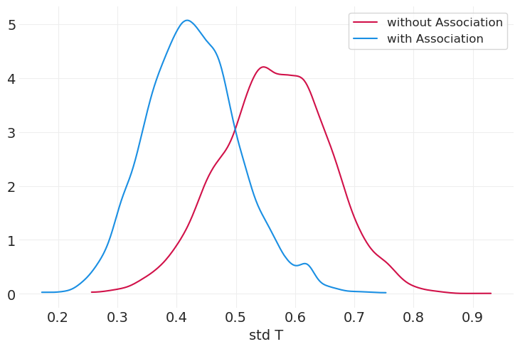
我们可以看到,包括给予和接受的参数减少了与社会关系相关的后验标准差。这是预期的,因为我们正在用这些额外的参数解释更多的方差。
模型系数#
_, ax = plt.subplots()
plt.sca(ax)
posterior = simulated_grf_inference.posterior


az.plot_dist(posterior["beta_G"], color="C0", label="$\\beta_G$")
plt.axvline(BETA_WG, color="C0", linestyle="--", label="True $\\beta_G$")

az.plot_dist(posterior["beta_R"], color="C1", label="$\\beta_R$")
plt.axvline(BETA_WR, color="C1", linestyle="--", label="True $\\beta_R$")

az.plot_dist(posterior["beta_A"], color="C2", label="$\\beta_A$")
plt.axvline(1, color="C2", linestyle="--", label="True $\\beta_A$")

plt.xlabel("posterior, $\\beta$")
plt.ylabel("density")
plt.legend();
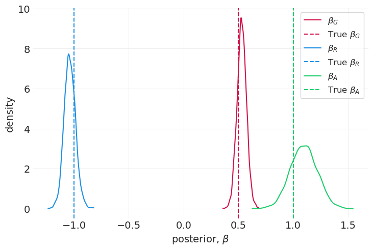
使用这个模型——它与数据模拟高度一致——我们能够从底层生成模型中恢复系数。
关联(在本例中为友谊)获得正系数 \(\beta_A\)。所有友谊关联都会导致给予
财富正向影响给予, \(\beta_G\)
财富负向影响接受 \(\beta_R\)
模型比较#
就交叉验证分数而言,控制正确的混淆因素可以提供更好的数据模型
az.compare(
    {"with confounds": simulated_grf_inference, "without confounds": simulated_gr_inference},
    var_name="G_AB",
)
| 排名 | elpd_loo | p_loo | elpd_diff | 权重 | 标准误 | dse | 警告 | 比例 | |
|---|---|---|---|---|---|---|---|---|---|
| 包含混淆因素 | 0 | -312.826182 | 39.968211 | 0.000000 | 1.000000e+00 | 18.536588 | 0.000000 | 真 | 对数 |
| 不包含混淆因素 | 1 | -326.921320 | 55.714152 | 14.095138 | 5.648815e-13 | 18.234868 | 4.638331 | 真 | 对数 |
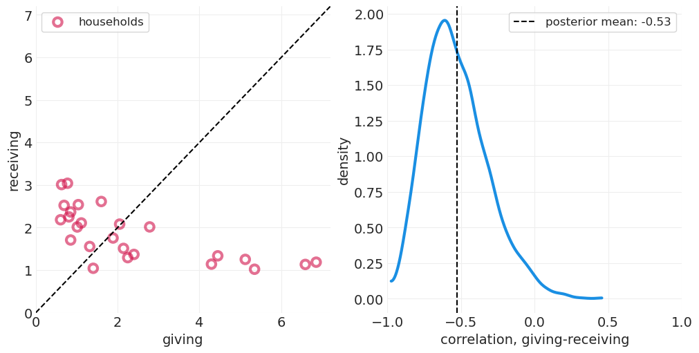
考虑混淆特征使社交网络抽象变得不那么重要#
plot_wealth_gifting_posterior(simulated_grf_inference, data_range=(0.4, 0.6))
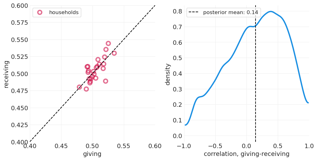
给予/接受主要由友谊和/或家庭财富解释,因此在考虑这些变量后,在 dyad 中定义的给予接受动态的信号较少
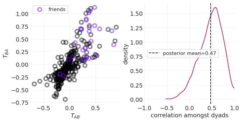
当控制正确的预测变量时,社会关系变得更加独立#
_, axs = plt.subplots(1, 2, figsize=(8, 4))
plt.sca(axs[0])
plot_posterior_household_ties(simulated_grf_inference, color_friends=True)

plt.sca(axs[1])
plot_posterior_reciprocity(simulated_grf_inference)
联合分布中的 x 形表示一组独立的变量。米
当考虑混淆因素时,大多数连接概率都在 0.5 左右#
这表明,在考虑友谊和财富之后,社会关系或多或少是随机的
plot_posterior_mean_graph(simulated_grf_inference)
将给予-接受特征模型拟合到真实数据#
在讲座中,McElreath 报告了真实数据的结果,但鉴于我手头的数据集版本,目前尚不清楚如何继续进行。
SHARING.head()
| hidA | hidB | did | giftsAB | giftsBA | offset | drel1 | drel2 | drel3 | drel4 | dlndist | dass | d0125 | |
|---|---|---|---|---|---|---|---|---|---|---|---|---|---|
| 0 | 1 | 2 | 1 | 0 | 4 | 0.000 | 0 | 0 | 1 | 0 | -2.790 | 0.000 | 0 |
| 1 | 1 | 3 | 2 | 6 | 31 | -0.003 | 0 | 1 | 0 | 0 | -2.817 | 0.044 | 0 |
| 2 | 1 | 4 | 3 | 2 | 5 | -0.019 | 0 | 1 | 0 | 0 | -1.886 | 0.025 | 0 |
| 3 | 1 | 5 | 4 | 4 | 2 | 0.000 | 0 | 1 | 0 | 0 | -1.892 | 0.011 | 0 |
| 4 | 1 | 6 | 5 | 8 | 2 | -0.003 | 1 | 0 | 0 | 0 | -3.499 | 0.022 | 0 |
为了拟合模型,我们需要知道真实数据集中的哪些列与以下内容相关联
关联指标 \(A_{AB}\)
家庭 A 的财富 \(W_A\)
家庭 B 的财富 \(W_B\)
查看数据集,尚不完全清楚我们应该/可以关联哪些列与这些变量中的每一个,以复制讲座中的图。也就是说,如果我们确实知道这些列——或者如何推导出它们——那么很容易通过以下方式拟合模型
>>> grf_model, grf_inference = fit_giving_receiving_features_model(SHARING)
# grf_model, grf_inference = fit_giving_receiving_features_model(SHARING)
额外的结构:三角形闭合#
关系倾向于以三元组形式出现
块模型 – 社会关系在社会群体内更常见
家庭
教室
实际的城市街区
添加额外的混淆因素
utils.draw_causal_graph(
    edge_list=[
        ("H_A", "G_AB"),
        ("H_B", "G_AB"),
        ("H_A", "T_AB"),
        ("H_B", "T_AB"),
        ("H_A", "T_BA"),
        ("H_B", "T_BA"),
        ("T_AB", "G_AB"),
        ("T_BA", "G_AB"),
        ("H_A", "K_A"),
        ("H_B", "K_B"),
        ("K_A", "T_AB"),
        ("K_B", "T_AB"),
        ("K_A", "T_BA"),
        ("K_B", "T_BA"),
    ],
    node_props={
        "T_AB": {"style": "dashed"},
        "T_BA": {"style": "dashed"},
        "K_A": {"color": "red", "label": "A's block membership"},
        "K_B": {"color": "red", "label": "B's block membership"},
        "unobserved": {"style": "dashed"},
    },
    edge_props={
        ("K_A", "T_AB"): {"color": "red"},
        ("K_A", "T_BA"): {"color": "red"},
        ("K_B", "T_AB"): {"color": "red"},
        ("K_B", "T_BA"): {"color": "red"},
    },
)

后验网络被正则化#
社交网络试图表达观察结果中的规律性
推断的网络是正则化的
块和聚类仍然是离散的子组,那么像年龄或空间距离这样的“连续聚类”呢?下一讲关于高斯过程的目标
def plot_gifting_graph(data, title=None, edge_colormap="gray_r", **plot_graph_kwargs):

    G = nx.DiGraph()
    edge_weights = []
    for ii, (A, B) in enumerate(DYADS):
        row = data.iloc[ii]

        if row.giftsAB > 0:
            A_, B_ = A, B
            weight = row.giftsAB

        if row.giftsBA > 0:
            A_, B_ = B, A
            weight = row.giftsBA

        G.add_edge(A, B, weight=weight)
        edge_weights.append(weight)

    edge_weights = np.array(edge_weights)
    edge_color = np.log(edge_weights)

    _, axs = plt.subplots(1, 2, figsize=(10, 5), width_ratios=[20, 1])
    plt.sca(axs[0])
    plt.set_cmap(edge_colormap)
    utils.plot_graph(G, edge_color=edge_color, pos=TIES_LAYOUT_POSITION, **plot_graph_kwargs)
    plt.title(title)

    # Fake axis to hold colorbar
    plt.sca(axs[1])
    axs[1].set_aspect(0.0001)
    axs[1].set_visible(False)
    img = plt.imshow(np.array([[edge_color.min(), edge_color.max()]]))
    img.set_visible(False)

    clb = plt.colorbar(orientation="vertical", fraction=0.8, pad=0.1)
    clb.set_label("log(# gifts)", rotation=90)
将送礼观察结果与在这些观察结果上训练的模型进行比较#
⚠️ 以下示例使用的是模拟数据
# Data that is modeled
edge_weight_cmap = "gray"  # switch colorscale to highlight sparsity
plot_gifting_graph(
    simulated_wealth_gifts, edge_colormap=edge_weight_cmap, alpha=1, title="Observed Gifting"
)

# Resulting model is sparser
plot_posterior_mean_graph(
    simulated_grf_inference,
    edge_colormap=edge_weight_cmap,
    alpha=1,
    title="Model Posterior Social Ties",
)
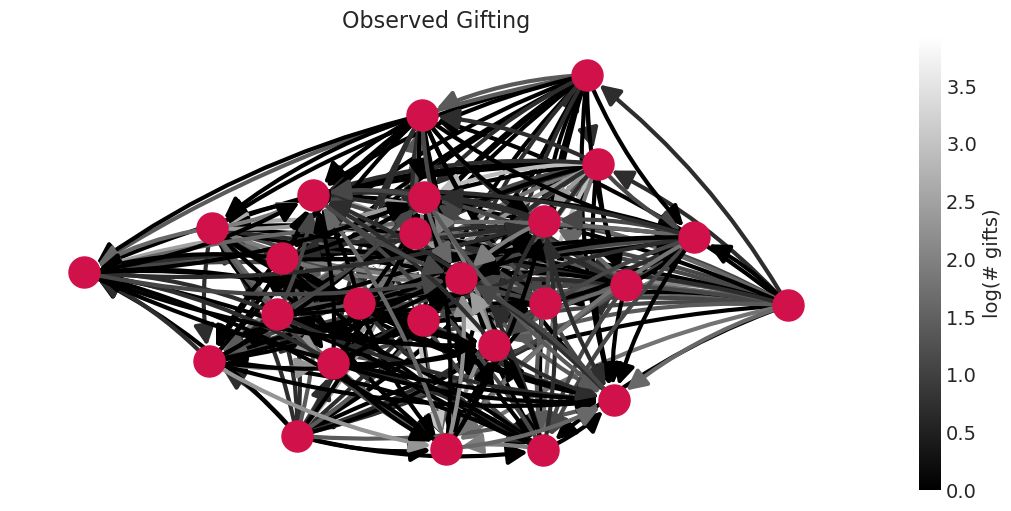
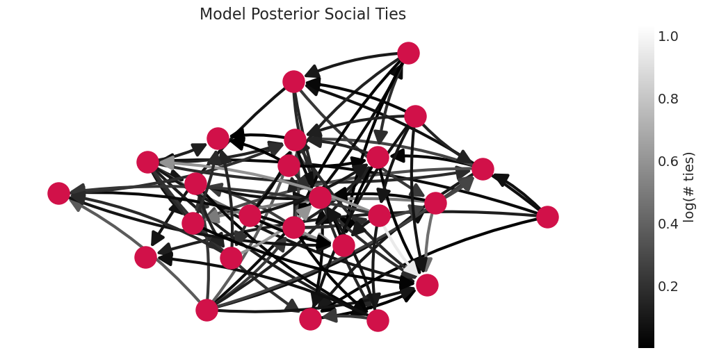
观察到的送礼网络比从数据估计的社会关系网络更密集,这表明模型的汇集正在向社会关系网络添加正则化(压缩)。
技术带来的变化影响#
社交网络试图表达观察数据中的规律性
因此,推断出的网络是正则化的,捕捉到那些结构化的规律性影响
当聚类不是离散的时会发生什么?
年龄、距离、空间位置
我们需要一种按“连续聚类”进行分层或执行局部汇集的方法
这就是高斯过程在下一讲中出现的原因。
允许我们解决需要系统发育和空间模型的问题
奖励:构造变量 \(\neq\) 分层#
确定性函数的输出,例如
身体质量指数:\(BMI = \frac{mass}{height^2}\)
“*人均”、“*单位时间”
一种常见的误解是,通过变量进行除法或重新缩放等同于控制该变量。
因果推断可以提供一种以更原则性的方式组合变量的方法。
示例:用人口除 GDP#
utils.draw_causal_graph(
    edge_list=[("P", "GDP/P"), ("GDP", "GDP/P"), ("P", "GDP")],
    node_props={
        "P": {"label": "population, P"},
        "GDP": {"label": "gross domestic product, GDP"},
    },
    edge_props={
        ("P", "GDP"): {
            "color": "red",
            "label": "assumed to be linear\n(not realistic)",
            "fontcolor": "red",
        }
    },
    graph_direction="LR",
)

假设人口线性地缩放 GDP
按人口划分不等同于按人口分层
utils.draw_causal_graph(
    edge_list=[("P", "GDP/P"), ("GDP", "GDP/P"), ("P", "GDP"), ("P", "X"), ("X", "GDP")],
    node_props={
        "X": {"color": "red", "label": "cause of interest, X"},
        "GDP": {"color": "red"},
    },
    edge_props={
        ("P", "X"): {"color": "blue", "label": "backdoor\npath", "fontcolor": "blue"},
        ("X", "GDP"): {"color": "red", "label": "Causal Path", "fontcolor": "red"},
        ("P", "GDP/P"): {"color": "blue"},
        ("GDP", "GDP/P"): {"color": "red"},
    },
    graph_direction="LR",
)

但情况更糟。在下面的场景中,我们想要估计 \(X\) 对 GDP/P 的因果效应,由 \(P\) 创建的分叉不会通过简单地计算 GDP/P 来消除
另一个示例:比率#
utils.draw_causal_graph(
    edge_list=[("T", "Y/T"), ("Y", "Y/T"), ("T", "Y"), ("X", "Y")], graph_direction="LR"
)

比率通常计算为 \(\frac{\text{事件数}}{\text{单位时间}}\) 并建模为结果
没有考虑不同时间量的不同精度
假设所有 Y/T 都具有相同的精度,尽管较大的 Y 通常有更多的时间发生,因此具有更高的精度
折叠为点估计会消除我们谈论比率不确定性的能力(例如,分布)
时间较少/精度较低的数据点与时间较长/精度较高的数据具有相同的估计可信度
按时间划分并不能控制时间
如果比率是科学问题的焦点,对计数进行建模(例如,泊松回归)以估计比率参数
另一个示例:差异分数#
utils.draw_causal_graph(
    edge_list=[("H0", "H1-H0"), ("H1", "H1-H0"), ("H0", "H1"), ("X", "H1")], graph_direction="LR"
)

例如,植物生长实验,其中 H0 和 H1 是植物的起始高度和结束高度,X 是抗真菌处理。
差异分数 H1-H0 对 H0 对 H1 的影响做出了强烈的假设,即
对于所有起始高度,生长效应都是恒定的
植物高度没有下限或上限效应
需要在 GLM(线性回归)的右侧对 H0 进行建模,因为它是 H1 的原因。这就是我们在植物生长示例中所做的
回顾:构造变量是不好的#
算术不是分层
隐含地假设原因之间存在固定的函数关系;你应该估计这些函数关系
通常忽略不确定性
使用残差作为新数据并不能控制变量;不要在因果推断中使用(尽管在预测设置中这样做很常见)
临时性#
具有直观理由的临时程序
“我们期望看到相关性”。
你为什么期望看到相关性(明确假设)?
另外,如果你没有看到相关性,为什么这意味着以该相关性为条件的某个 NULL 被证伪了?
如果一个临时程序确实有效(它们有时可能是偶然正确的),则需要通过因果逻辑和测试来证明其合理性
简单规则:对你测量的东西进行建模
不要尝试对从度量导出的新指标进行建模
许可声明#
本示例库中的所有笔记本均根据 MIT 许可证 提供,该许可证允许修改和再分发以用于任何用途,前提是保留版权和许可声明。
引用 PyMC 示例#
要引用此笔记本,请使用 Zenodo 为 pymc-examples 存储库提供的 DOI。
重要提示
许多笔记本改编自其他来源:博客、书籍…… 在这种情况下,您也应该引用原始来源。
另请记住引用您的代码使用的相关库。
这是一个 bibtex 中的引用模板
@incollection{citekey,
  author    = "<notebook authors, see above>",
  title     = "<notebook title>",
  editor    = "PyMC Team",
  booktitle = "PyMC examples",
  doi       = "10.5281/zenodo.5654871"
}
一旦渲染,它可能看起来像
社交网络#
本笔记本是 PyMC 移植的 Statistical Rethinking 2023 Richard McElreath 讲座系列的一部分。
视频 - 第 15 讲 - 社交网络# 第 15 讲 - 社交网络