高斯过程

此笔记本是 PyMC 端口的一部分，该端口移植了 Richard McElreath 的统计再思考 2023系列讲座。

视频 - 第 16 讲 - 高斯过程# 第 16 讲 - 高斯过程

# Ignore warnings
import warnings

import arviz as az
import numpy as np
import pandas as pd
import pymc as pm
import statsmodels.formula.api as smf
import utils as utils
import xarray as xr

from matplotlib import pyplot as plt
from matplotlib import style
from scipy import stats as stats

warnings.filterwarnings("ignore")

# Set matplotlib style
STYLE = "statistical-rethinking-2023.mplstyle"
style.use(STYLE)

返回海洋技术数据集

现在我们已经掌握了一些更高级的统计工具，我们将处理一些我们忽略的混淆因素

KLINE = utils.load_data("Kline2")
KLINE

	文化	人口	接触	工具总数	平均 TU	纬度	经度	经度2	人口对数
0	马莱库拉岛	1100	低	13	3.2	-16.3	167.5	-12.5	7.003065
1	提科皮亚岛	1500	低	22	4.7	-12.3	168.8	-11.2	7.313220
2	圣克鲁斯群岛	3600	低	24	4.0	-10.7	166.0	-14.0	8.188689
3	雅浦岛	4791	高	43	5.0	9.5	138.1	-41.9	8.474494
4	劳群岛	7400	高	33	5.0	-17.7	178.1	-1.9	8.909235
5	特罗布里恩群岛	8000	高	19	4.0	-8.7	150.9	-29.1	8.987197
6	楚克群岛	9200	高	40	3.8	7.4	151.6	-28.4	9.126959
7	马努斯岛	13000	低	28	6.6	-2.1	146.9	-33.1	9.472705
8	汤加	17500	高	55	5.4	-21.2	-175.2	4.8	9.769956
9	夏威夷	275000	低	71	6.6	19.9	-155.6	24.4	12.524526

utils.draw_causal_graph(
    edge_list=[("P", "T"), ("C", "T"), ("U", "T"), ("U", "P")],
    node_props={"U": {"style": "dashed"}, "unobserved": {"style": "dashed"}},
)

• 社会中的工具总数 \(T\) (结果)

• 人口 \(P\) (处理)

• 接触水平 \(C\)

• 未观察到的混淆因素 \(U\)，例如

  • 材料

  • 天气

应该存在空间协变

• 彼此靠近的岛屿应该具有相似的未观察到的混淆因素

• 岛屿应该共享历史背景

• 我们不必知道背景的确切动态，我们可以在宏观尺度上进行统计处理

技术创新/损失模型回顾

• 源自差分方程的稳态 \(\Delta T = \alpha P^ \beta - \gamma T\)

  • \(\alpha\) 是创新率

  • \(P\) 是人口

  • \(\beta\) 是弹性率（收益递减）

  • \(\gamma\) 是随时间推移的损失（例如，遗忘）率

• 提供长期预期的工具数量

  • \(\hat T = \frac{\alpha P ^ \beta}{\gamma}\)

  • 使用 \(\lambda= \hat T\) 作为 \(\text{Poisson}(\lambda)\) 分布的预期速率参数

• 我们如何在模型中编码空间协方差？

让我们从一个更简单的忽略人口的模型开始

\[\begin{split} \begin{align*} T_i &\sim \text{Poisson}(\lambda_i) \\ \lambda_i &= \bar \alpha + \alpha_{S[i]} \\ \begin{pmatrix} \alpha_1 \\ \alpha_2 \\ \vdots \\ \alpha_{10} \end{pmatrix} &= \text{MVNormal} \left( \begin{bmatrix} 0 \\ 0 \\ \vdots \\ 0 \end{bmatrix}, \textbf{K} \right) \end{align*} \end{split}\]

• \(\alpha_{S[i]}\) 是每个社会的可变截距

  • 这些将基于它们彼此之间的空间距离而具有协变

  • 更接近的社会具有相似的偏移

• \(\mathbf{K}\) 社会之间的协方差

  • 将协方差建模为距离的函数

  • 虽然 \(\mathbf{K}\) 有很多参数（45 个协方差），但我们应该能够利用空间规律性来估计少得多的有效参数。这很好，因为我们只有 10 个数据点 😅

高斯过程（抽象概念）

• 使用核函数生成协方差矩阵

  • 需要的参数远少于协方差矩阵条目

  • 可以生成任何维度的协方差矩阵（即“MNNormal的无限维推广”）

  • 可以生成任何点的预测

• 核函数基于比较指标（例如）计算两个点的协方差

  • 空间距离

  • 时间差

  • 年龄差

不同的核函数

def plot_kernel_function(
    kernel_function, max_distance=1, resolution=100, label=None, ax=None, **line_kwargs
):
    """Helper to plot a kernel function"""
    X = np.linspace(0, max_distance, resolution)[:, None]
    covariance = kernel_function(X, X)
    distances = np.linspace(0, max_distance, resolution)
    if ax is not None:
        plt.sca(ax)
    utils.plot_line(distances, covariance[0, :], label=label, **line_kwargs)
    plt.xlim([0, max_distance])
    plt.ylim([-0.05, 1.05])
    plt.xlabel("|X1-X2|")
    plt.ylabel("covariance")
    if label is not None:
        plt.legend()

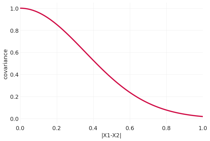
二次 (L2) 核函数

• 又名 RGB

• 又名高斯核

\[ K(x_i, x_j) = \eta^2 \exp \left(- \frac{(x_i - x_j)^2}{\sigma^2} \right) \]

def quadratic_distance_kernel(X0, X1, eta=1, sigma=0.5):
    # Use linear algebra identity: ||x-y||^2 = ||x||^2 + ||y||^2 - 2 * x^T * y
    X0_norm = np.sum(X0**2, axis=-1)
    X1_norm = np.sum(X1**2, axis=-1)
    squared_distances = X0_norm[:, None] + X1_norm[None, :] - 2 * X0 @ X1.T
    rho = 1 / sigma**2
    return eta**2 * np.exp(-rho * squared_distances)


plot_kernel_function(quadratic_distance_kernel)

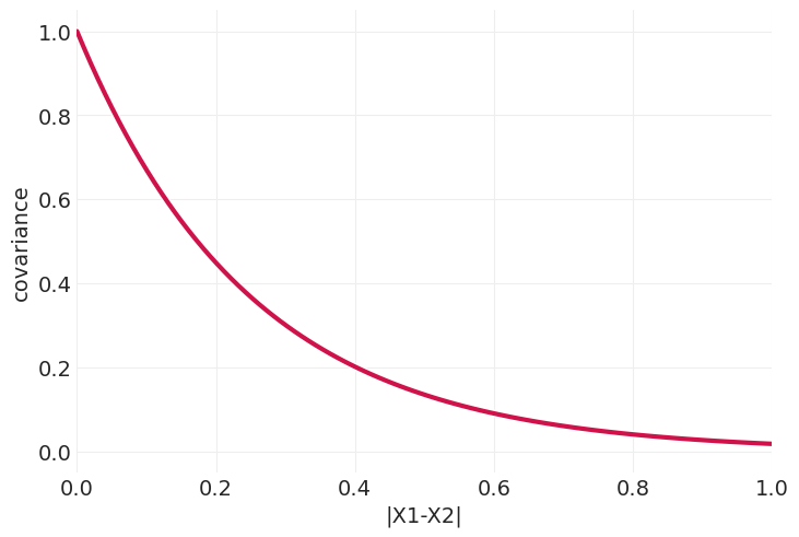
奥恩斯坦-乌伦贝克核

\[\begin{split} \begin{align*} K(x_i, x_j) &= \eta^2 \exp \left(- \frac{|x_i - x_j|}{\sigma} \right) \\ \sigma &= \frac{1}{\rho} \end{align*} \end{split}\]

def ornstein_uhlenbeck_kernel(X0, X1, eta_squared=1, rho=4):
    distances = np.abs(X1[None, :] - X0[:, None])
    return eta_squared * np.exp(-rho * distances)


plot_kernel_function(ornstein_uhlenbeck_kernel)

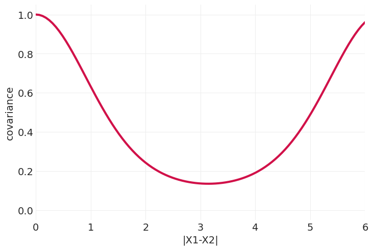
周期核

\[ K(x_i, x_j) = \eta^2 \exp \left(- \frac{\sin^2((x_i - x_j) / p)}{\sigma^2} \right) \]

具有额外的周期性参数 \(p\)

def periodic_kernel(X0, X1, eta=1, sigma=1, periodicity=0.5):
    distances = np.sin((X1[None, :] - X0[:, None]) * periodicity) ** 2
    rho = 2 / sigma**2
    return eta**2 * np.exp(-rho * distances)


plot_kernel_function(periodic_kernel, max_distance=6)

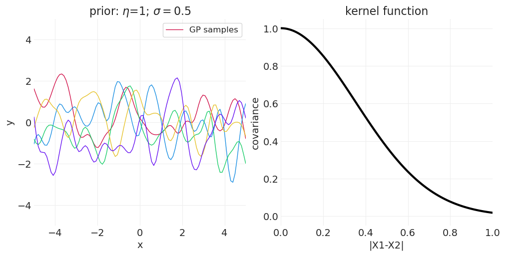
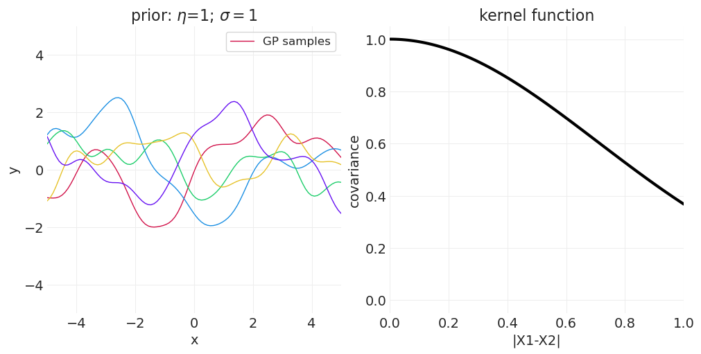
高斯过程先验

使用高斯/L2 核函数生成我们的协方差 \(\mathbf{K}\)，我们可以调整一些参数

• 改变 \(\sigma\) 控制核函数的带宽

  • 较小的 \(\sigma\) 使协方差随空间快速衰减

  • 较大的 \(\sigma\) 允许协方差扩展到更大的距离

• 改变 \(\eta\) 控制最大协方差程度

一维示例

下面我们从一维高斯过程中绘制函数，改变 \(\sigma\) 或 \(\eta\) 以演示参数对样本空间相关性的影响。

# Helper functions
def plot_gaussian_process(
    X, samples=None, mean=None, cov=None, X_obs=None, Y_obs=None, uncertainty_prob=0.89
):
    X = X.ravel()

    # Plot GP samples
    for ii, sample in enumerate(samples):
        label = "GP samples" if not ii else None
        utils.plot_line(X, sample, color=f"C{ii}", linewidth=1, label=label)

    # Add GP mean, if provided
    if mean is not None:
        mean = mean.ravel()
        utils.plot_line(X, mean, color="k", label="GP mean")

        # Add uncertainty around mean; requires covariance matrix
        if cov is not None:
            z = stats.norm.ppf(1 - (1 - uncertainty_prob) / 2)
            uncertainty = z * np.sqrt(np.diag(cov))
            plt.fill_between(
                X,
                mean + uncertainty,
                mean - uncertainty,
                alpha=0.1,
                color="gray",
                zorder=1,
                label="GP uncertainty",
            )

    # Add any training data points, if provided
    if X_obs is not None:
        utils.plot_scatter(X_obs, Y_obs, color="k", label="observations", zorder=100, alpha=1)

    plt.xlim([X.min(), X.max()])
    plt.ylim([-5, 5])
    plt.xlabel("x")
    plt.ylabel("y")
    plt.legend()


def plot_gaussian_process_prior(kernel_function, n_samples=3, figsize=(10, 5), resolution=100):
    X = np.linspace(-5, 5, resolution)[:, None]

    prior = gaussian_process_prior(X, kernel_function)
    samples = prior.rvs(n_samples)

    _, axs = plt.subplots(1, 2, figsize=figsize)
    plt.sca(axs[0])
    plot_gaussian_process(X, samples=samples)

    plt.sca(axs[1])
    plot_kernel_function(kernel_function, color="k")
    plt.title(f"kernel function")
    return axs


def gaussian_process_prior(X_pred, kernel_function):
    """Initializes a Gaussian Process prior distribution for provided Kernel function"""
    mean = np.zeros(X_pred.shape).ravel()
    cov = kernel_function(X_pred, X_pred)
    return stats.multivariate_normal(mean=mean, cov=cov, allow_singular=True)

改变 \(\sigma\)

from functools import partial

eta = 1
for sigma in [0.25, 0.5, 1]:
    kernel_function = partial(quadratic_distance_kernel, eta=eta, sigma=sigma)
    axs = plot_gaussian_process_prior(kernel_function, n_samples=5)
    axs[0].set_title(f"prior: $\\eta$={eta}; $\\sigma=${sigma}")

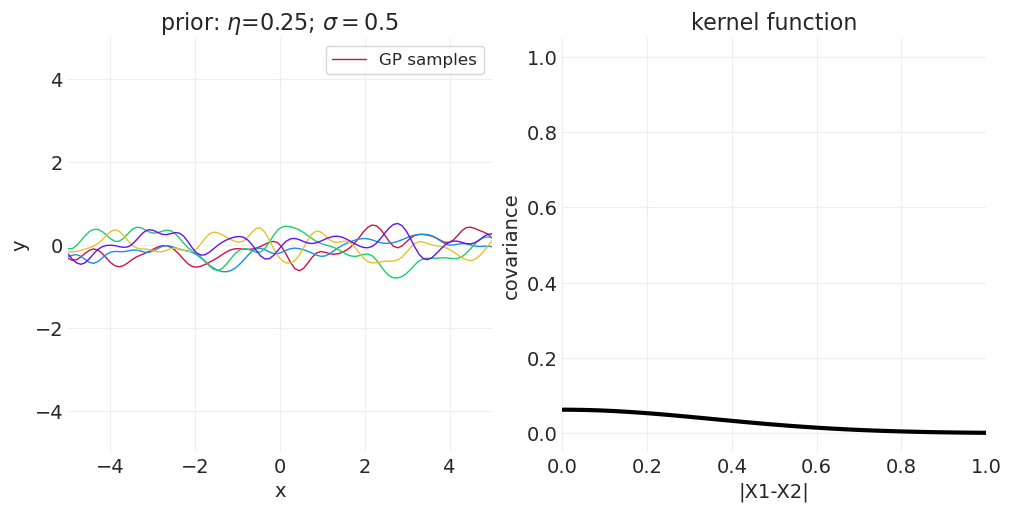
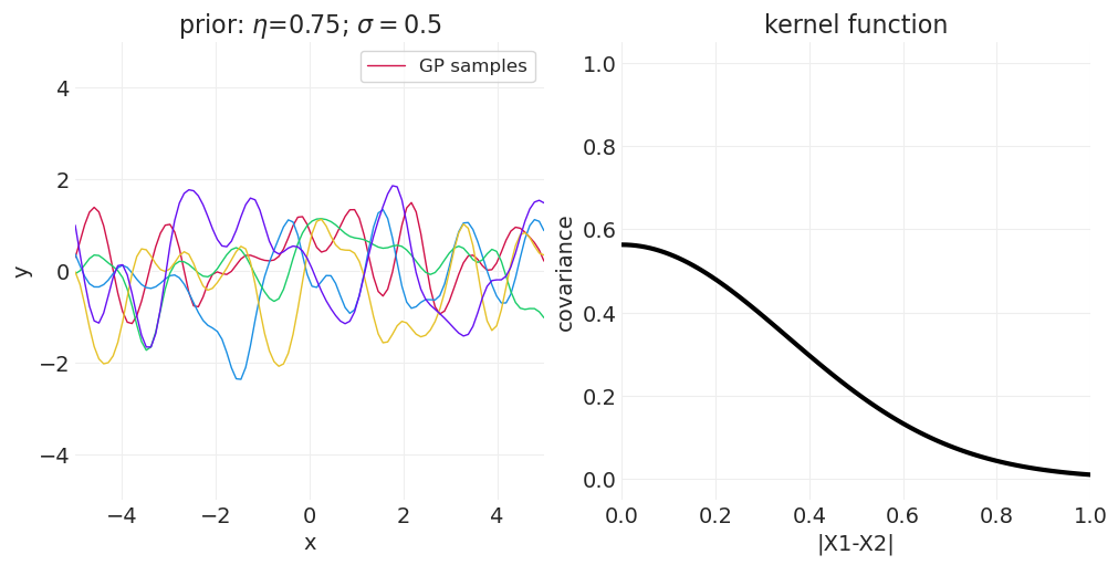
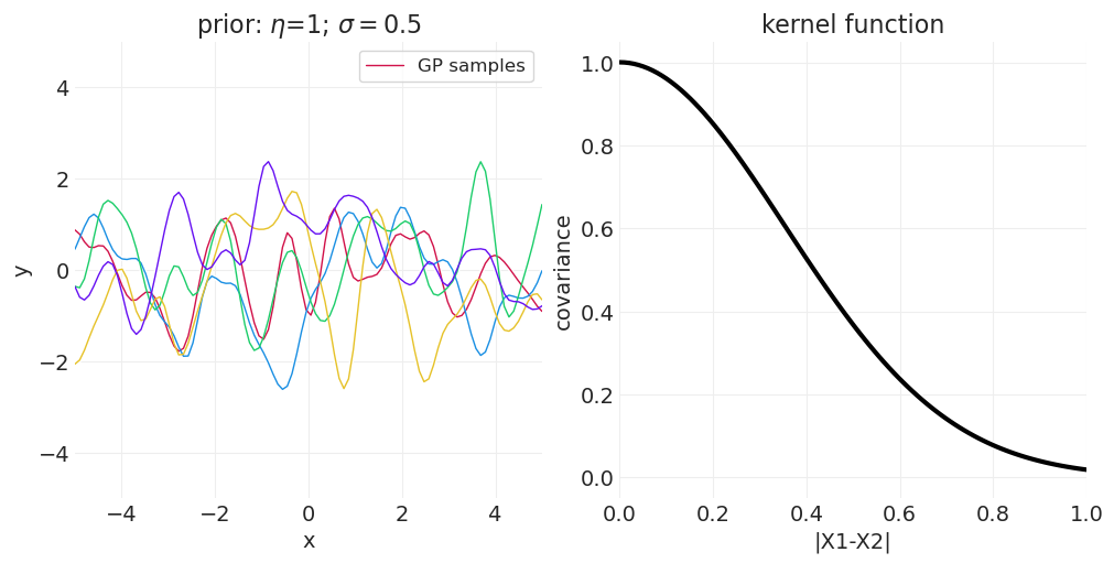
改变 \(\eta\)

sigma = 0.5
for eta in [0.25, 0.75, 1]:
    kernel_function = partial(quadratic_distance_kernel, eta=eta, sigma=sigma)
    axs = plot_gaussian_process_prior(kernel_function, n_samples=5)
    axs[0].set_title(f"prior: $\\eta$={eta}; $\\sigma=${sigma}")

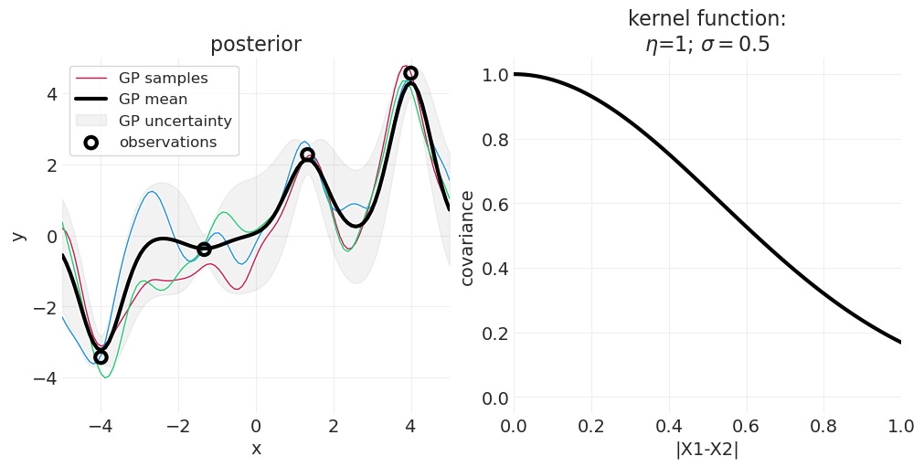
高斯过程后验

当模型观察到数据时，它会调整后验以考虑该数据，同时还结合先验的平滑度约束。

def gaussian_process_posterior(
    X_obs, Y_obs, X_pred, kernel_function, sigma_y=1e-6, smoothing_factor=1e-6
):
    """Initializes a Gaussian Process Posterior distribution"""

    # Observation covariance
    K_obs = kernel_function(X_obs, X_obs)
    K_obs_noise = sigma_y**2 * np.eye(len(X_obs))
    K_obs += K_obs_noise
    K_obs_inv = np.linalg.inv(K_obs)

    # Prediction grid covariance
    K_pred = kernel_function(X_pred, X_pred)
    K_pred_smooth = smoothing_factor * np.eye(len(X_pred))
    K_pred += K_pred_smooth

    # Covariance between observations and prediction grid
    K_obs_pred = kernel_function(X_obs, X_pred)

    # Posterior
    posterior_mean = K_obs_pred.T.dot(K_obs_inv).dot(Y_obs)
    posterior_cov = K_pred - K_obs_pred.T.dot(K_obs_inv).dot(K_obs_pred)

    return stats.multivariate_normal(
        mean=posterior_mean.ravel(), cov=posterior_cov, allow_singular=True
    )


def plot_gaussian_process_posterior(
    X_obs,
    Y_obs,
    X_pred,
    kernel_function,
    sigma_y=1e-6,
    n_samples=3,
    figsize=(10, 5),
    resolution=100,
):
    X = np.linspace(-5, 5, resolution)[:, None]

    posterior = gaussian_process_posterior(X_obs, Y_obs, X, kernel_function, sigma_y=sigma_y)
    samples = posterior.rvs(n_samples)

    _, axs = plt.subplots(1, 2, figsize=figsize)
    plt.sca(axs[0])

    plot_gaussian_process(
        X_pred,
        samples=posterior.rvs(size=n_samples),
        mean=posterior.mean,
        cov=posterior.cov,
        X_obs=X_obs,
        Y_obs=Y_obs,
    )

    plt.sca(axs[1])
    plot_kernel_function(kernel_function, color="k")
    plt.title(f"kernel function")
    return axs

# Generate some training data
X_pred = np.linspace(-5, 5, 100)[:, None]
X_obs = np.linspace(-4, 4, 4)[:, None]
Y_obs = np.sin(X_obs) ** 2 + X_obs

# Initialize the kernel function
sigma_y = 0.25
sigma_kernel = 0.75
eta_kernel = 1
kernel_function = partial(quadratic_distance_kernel, eta=eta_kernel, sigma=sigma_kernel)

# Plot posterior
axs = plot_gaussian_process_posterior(
    X_obs, Y_obs, X_pred, kernel_function, sigma_y=sigma_y, n_samples=3
)
axs[0].set_title(f"posterior")
axs[1].set_title(f"kernel function:\n$\\eta$={eta}; $\\sigma=${sigma}");

基于距离的模型

\[\begin{split} \begin{align} T_i &\sim \text{Poisson}(\lambda_i) \\ \log(\lambda_i) &= \bar \alpha + \alpha_{S[i]} \\ \begin{pmatrix} \alpha_1 \\ \alpha_2 \\ \vdots \\ \alpha_{10} \end{pmatrix} &= \text{MVNormal}\left( \begin{bmatrix} 0 \\ 0 \\ \vdots \\ 0 \end{bmatrix}, \textbf{K} \right) \\ k_{i,j} &= \eta^2\exp(-\rho^2D_{i,j}^2)) \\ \eta^2 &\sim \text{Exponential}(2) \\ \rho^2 &\sim \text{Exponential}(0.5) \end{align} \end{split}\]

岛屿距离矩阵

# Distance matrix D_{i, j}
ISLANDS_DISTANCE_MATRIX = utils.load_data("islands_distance_matrix")
ISLANDS_DISTANCE_MATRIX.set_index(ISLANDS_DISTANCE_MATRIX.columns, inplace=True)
ISLANDS_DISTANCE_MATRIX.style.format(precision=1).background_gradient(cmap="viridis").set_caption(
    "Distance in Thousands of km"
)

距离单位：千公里

	马莱库拉岛	提科皮亚岛	圣克鲁斯群岛	雅浦岛	劳群岛	特罗布里恩群岛	楚克群岛	马努斯岛	汤加	夏威夷
马莱库拉岛	0.0	0.5	0.6	4.4	1.2	2.0	3.2	2.8	1.9	5.7
提科皮亚岛	0.5	0.0	0.3	4.2	1.2	2.0	2.9	2.7	2.0	5.3
圣克鲁斯群岛	0.6	0.3	0.0	3.9	1.6	1.7	2.6	2.4	2.3	5.4
雅浦岛	4.4	4.2	3.9	0.0	5.4	2.5	1.6	1.6	6.1	7.2
劳群岛	1.2	1.2	1.6	5.4	0.0	3.2	4.0	3.9	0.8	4.9
特罗布里恩群岛	2.0	2.0	1.7	2.5	3.2	0.0	1.8	0.8	3.9	6.7
楚克群岛	3.2	2.9	2.6	1.6	4.0	1.8	0.0	1.2	4.8	5.8
马努斯岛	2.8	2.7	2.4	1.6	3.9	0.8	1.2	0.0	4.6	6.7
汤加	1.9	2.0	2.3	6.1	0.8	3.9	4.8	4.6	0.0	5.0
夏威夷	5.7	5.3	5.4	7.2	4.9	6.7	5.8	6.7	5.0	0.0

# Data / coords
CULTURE_ID, CULTURE = pd.factorize(KLINE.culture.values)
ISLAND_DISTANCES = ISLANDS_DISTANCE_MATRIX.values.astype(float)
TOOLS = KLINE.total_tools.values.astype(int)
coords = {"culture": CULTURE}

with pm.Model(coords=coords) as distance_model:

    # Priors
    alpha_bar = pm.Normal("alpha_bar", 3, 0.5)
    eta_squared = pm.Exponential("eta_squared", 2)
    rho_squared = pm.Exponential("rho_squared", 0.5)

    # Gaussian Process
    kernel_function = eta_squared * pm.gp.cov.ExpQuad(input_dim=1, ls=rho_squared)
    GP = pm.gp.Latent(cov_func=kernel_function)
    alpha = GP.prior("alpha", X=ISLAND_DISTANCES, dims="culture")

    # Likelihood
    lambda_T = pm.math.exp(alpha_bar + alpha[CULTURE_ID])
    pm.Poisson("T", lambda_T, dims="culture", observed=TOOLS)

pm.model_to_graphviz(distance_model)

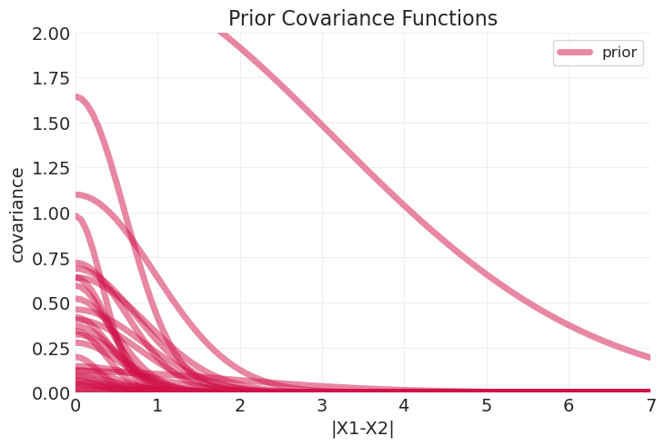
使用先验预测模拟检查模型

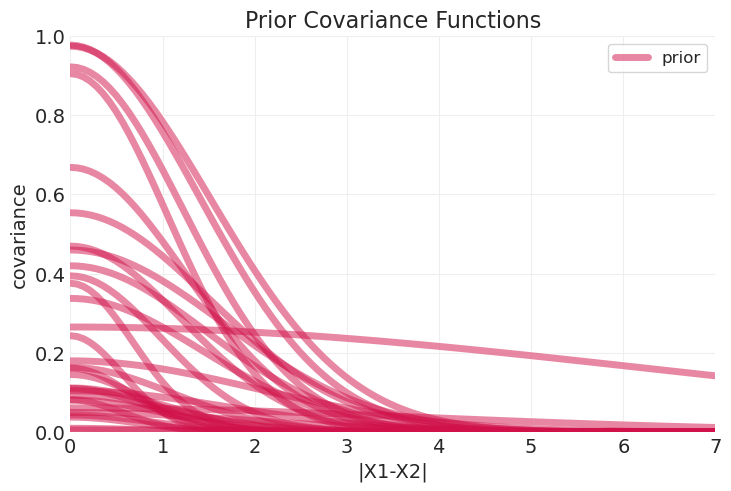
def plot_predictive_covariance(predictive, n_samples=30, color="C0", label=None):

    eta_samples = predictive["eta_squared"].values[0, :n_samples] ** 0.5
    sigma_samples = 1 / predictive["rho_squared"].values[0, :n_samples] ** 0.5

    for ii, (eta, sigma) in enumerate(zip(eta_samples, sigma_samples)):
        label = label if ii == 0 else None

        kernel_function = partial(quadratic_distance_kernel, eta=eta, sigma=sigma)
        plot_kernel_function(
            kernel_function, color=color, label=label, alpha=0.5, linewidth=5, max_distance=7
        )

with distance_model:
    prior_predictive = pm.sample_prior_predictive(random_seed=12).prior

plot_predictive_covariance(prior_predictive, label="prior")
plt.ylim([0, 2])
plt.title("Prior Covariance Functions");

Sampling: [T, alpha_bar, alpha_rotated_, eta_squared, rho_squared]

对数据建模

with distance_model:
    distance_inference = pm.sample(target_accept=0.99)

Initializing NUTS using jitter+adapt_diag...
Multiprocess sampling (4 chains in 4 jobs)
NUTS: [alpha_bar, eta_squared, rho_squared, alpha_rotated_]

Sampling 4 chains for 1_000 tune and 1_000 draw iterations (4_000 + 4_000 draws total) took 18 seconds.
The effective sample size per chain is smaller than 100 for some parameters.  A higher number is needed for reliable rhat and ess computation. See https://arxiv.org/abs/1903.08008 for details

az.summary(distance_inference, var_names=["~alpha_rotated_"])

	均值	标准差	hdi_3%	hdi_97%	mcse_mean	mcse_sd	ess_bulk	ess_tail	r_hat
alpha[马莱库拉岛]	-0.677	0.310	-1.273	-0.114	0.008	0.006	1471.0	1306.0	1.00
alpha[提科皮亚岛]	-0.297	0.275	-0.811	0.221	0.007	0.005	1561.0	2070.0	1.00
alpha[圣克鲁斯群岛]	-0.221	0.270	-0.714	0.299	0.007	0.005	1543.0	2215.0	1.00
alpha[雅浦岛]	0.326	0.261	-0.164	0.805	0.008	0.006	1238.0	1457.0	1.00
alpha[劳群岛]	0.077	0.264	-0.414	0.593	0.007	0.005	1413.0	1749.0	1.00
alpha[特罗布里恩群岛]	-0.280	0.339	-0.850	0.418	0.021	0.015	307.0	271.0	1.01
alpha[楚克群岛]	0.240	0.262	-0.243	0.741	0.007	0.005	1560.0	1828.0	1.00
alpha[马努斯岛]	-0.056	0.286	-0.621	0.456	0.010	0.007	979.0	742.0	1.00
alpha[汤加]	0.484	0.268	-0.007	1.008	0.009	0.006	1010.0	676.0	1.00
alpha[夏威夷]	0.811	0.246	0.348	1.275	0.007	0.005	1383.0	1662.0	1.00
alpha_bar	3.402	0.220	2.973	3.805	0.007	0.005	1122.0	1244.0	1.00
eta_squared	0.379	0.257	0.074	0.814	0.010	0.007	900.0	1114.0	1.00
rho_squared	0.293	0.521	0.000	1.233	0.051	0.036	158.0	134.0	1.01

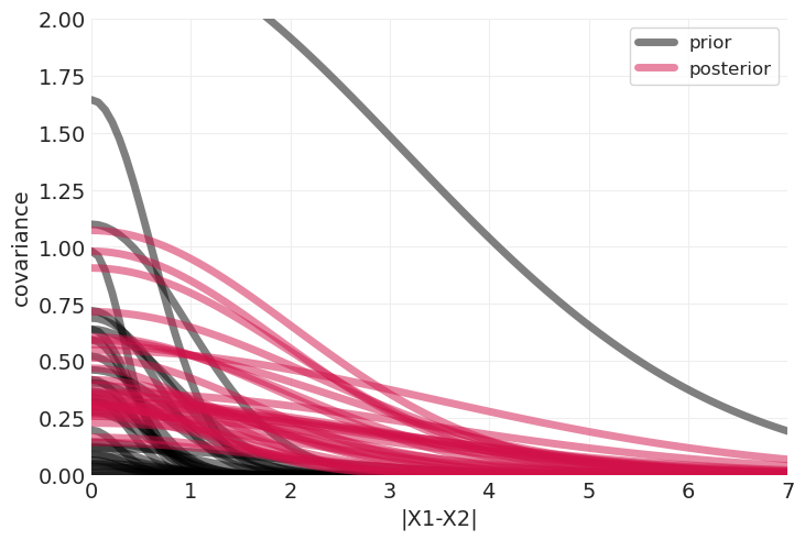
后验预测

将先验与后验进行比较

确保我们学到了一些东西

plot_predictive_covariance(prior_predictive, color="k", label="prior")
plot_predictive_covariance(distance_inference.posterior, label="posterior")
plt.ylim([0, 2]);

def distance_to_covariance(distance, eta_squared, rho_squared):
    return eta_squared * np.exp(-rho_squared * distance**2)


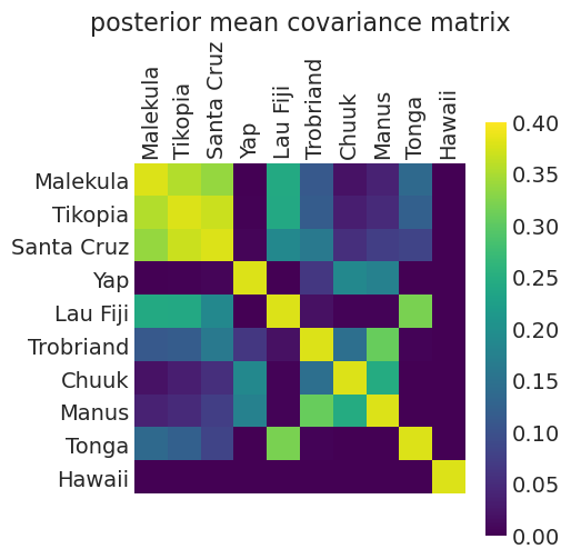
def calculate_posterior_mean_covariance_matrix(inference):
    posterior_mean = inference.posterior.mean(dim=("chain", "draw"))

    posterior_eta_squared = posterior_mean["eta_squared"].values
    posterior_rho_squared = posterior_mean["rho_squared"].values

    print("Posterior Mean Kernel parameters:")
    print("eta_squared:", posterior_eta_squared)
    print("rho_squared:", posterior_rho_squared)

    model_covariance = np.zeros_like(ISLANDS_DISTANCE_MATRIX).astype(float)
    for ii in range(10):
        for jj in range(10):
            model_covariance[ii, jj] = distance_to_covariance(
                ISLAND_DISTANCES[ii, jj],
                eta_squared=posterior_eta_squared,
                rho_squared=posterior_rho_squared,
            )

    return model_covariance


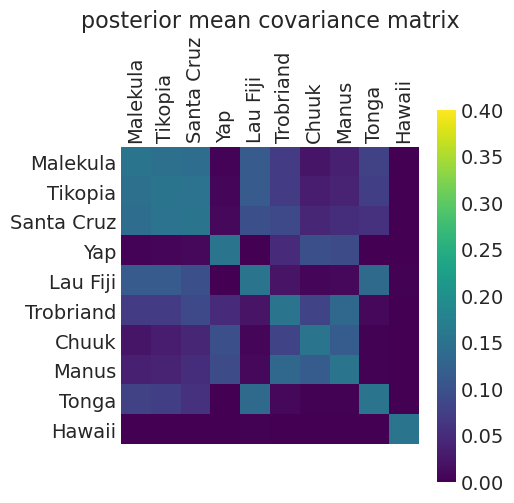
def plot_posterior_mean_covariance_matrix(covariance_matrix, clim=(0, 0.4)):
    plt.matshow(covariance_matrix)
    plt.xticks(np.arange(10), labels=KLINE.culture, rotation=90)
    plt.yticks(np.arange(10), labels=KLINE.culture)
    plt.clim(clim)
    plt.grid(False)
    plt.colorbar()
    plt.title("posterior mean covariance matrix");

distance_model_covariance = calculate_posterior_mean_covariance_matrix(distance_inference)
plot_posterior_mean_covariance_matrix(distance_model_covariance)

Posterior Mean Kernel parameters:
eta_squared: 0.3787328036103038
rho_squared: 0.2930628945484335

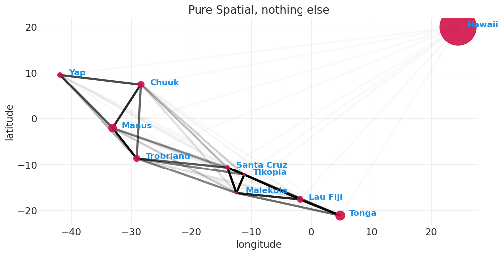
def plot_kline_model_covarance(covariance_matric, min_alpha=0.01, alpha_gain=1, max_cov=None):
    plt.subplots(figsize=(10, 5))
    # Plot covariance
    max_cov = covariance_matric.max() if max_cov is None else max_cov
    for ii in range(10):
        for jj in range(10):
            if ii != jj:
                lat_a = KLINE.loc[ii, "lat"]
                lon_a = KLINE.loc[ii, "lon2"]

                lat_b = KLINE.loc[jj, "lat"]
                lon_b = KLINE.loc[jj, "lon2"]
                cov = covariance_matric[ii, jj]
                alpha = (min_alpha + (1 - min_alpha) * (cov / max_cov)) ** (1 / alpha_gain)
                plt.plot((lon_a, lon_b), (lat_a, lat_b), linewidth=3, color="k", alpha=alpha)

    plt.scatter(KLINE.lon2, KLINE.lat, s=KLINE.population * 0.01, zorder=10, alpha=0.9)

    # Annotate
    for ii in range(10):
        plt.annotate(
            KLINE.loc[ii, "culture"],
            (KLINE.loc[ii, "lon2"] + 1.5, KLINE.loc[ii, "lat"]),
            zorder=11,
            color="C1",
            fontsize=12,
            fontweight="bold",
        )
    plt.xlabel("longitude")
    plt.ylabel("latitude")
    plt.axis("tight")


plot_kline_model_covarance(distance_model_covariance, max_cov=0.4)
plt.title("Pure Spatial, nothing else");

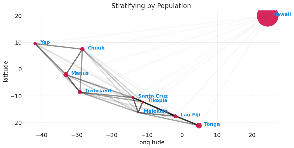
按人口规模分层

\[\begin{split} \begin{align} T_i &\sim \text{Poisson}(\lambda_i) \\ \lambda_i &= \frac{\bar \alpha P^\beta}{\gamma} \exp(\alpha_{S[i]}) \\ \begin{pmatrix} \alpha_1 \\ \alpha_2 \\ \vdots \\ \alpha_{10} \end{pmatrix} &= \text{MVNormal} \left( \begin{bmatrix} 0 \\ 0 \\ \vdots \\ 0 \end{bmatrix}, \textbf{K} \right) \\ k_{i,j} &= \eta^2\exp(-\rho^2D_{i,j}^2)) \\ \bar \alpha, \beta, \gamma &\sim \text{Exponential}(1) \\ \eta^2 &\sim \text{Exponential}(2) \\ \rho^2 &\sim \text{Exponential}(0.5) \end{align} \end{split}\]

• 我们现在将稳态方程折叠到截距/基线工具方程中

• 包含一个额外的 \(\exp\) 乘数来处理社会层面的偏移。这里的想法是

  • 如果 \(\alpha_{S[i]}=0\)，那么该社会是平均水平，我们回退到差分方程的期望值，即乘数为 1

  • 如果 \(\alpha_{S[i]}>0\)，则工具生产得到提升。这种提升在空间上邻近的社会之间共享

with pm.Model(coords=coords) as distance_population_model:

    population = pm.Data("log_population", KLINE.logpop.values.astype(float))
    CULTURE_ID_ = pm.Data("CULTURE_ID", CULTURE_ID)

    # Priorsdistancesdistances
    alpha_bar = pm.Exponential("alpha_bar", 1)
    gamma = pm.Exponential("gamma", 1)
    beta = pm.Exponential("beta", 1)
    eta_squared = pm.Exponential("eta_squared", 2)
    rho_squared = pm.Exponential("rho_squared", 2)

    # Gaussian Process
    kernel_function = eta_squared * pm.gp.cov.ExpQuad(input_dim=1, ls=rho_squared)
    GP = pm.gp.Latent(cov_func=kernel_function)
    alpha = GP.prior("alpha", X=ISLAND_DISTANCES, dims="culture")

    # Likelihood
    lambda_T = (alpha_bar / gamma * population[CULTURE_ID_] ** beta) * pm.math.exp(
        alpha[CULTURE_ID_]
    )
    pm.Poisson("T", lambda_T, observed=TOOLS, dims="culture")

pm.model_to_graphviz(distance_population_model)

先验预测

with distance_population_model:
    prior_predictive = pm.sample_prior_predictive(random_seed=12).prior

plot_predictive_covariance(prior_predictive, label="prior")
plt.ylim([0, 1])
plt.title("Prior Covariance Functions");

Sampling: [T, alpha_bar, alpha_rotated_, beta, eta_squared, gamma, rho_squared]

with distance_population_model:
    distance_population_inference = pm.sample(target_accept=0.99)

Initializing NUTS using jitter+adapt_diag...
Multiprocess sampling (4 chains in 4 jobs)
NUTS: [alpha_bar, gamma, beta, eta_squared, rho_squared, alpha_rotated_]

Sampling 4 chains for 1_000 tune and 1_000 draw iterations (4_000 + 4_000 draws total) took 82 seconds.

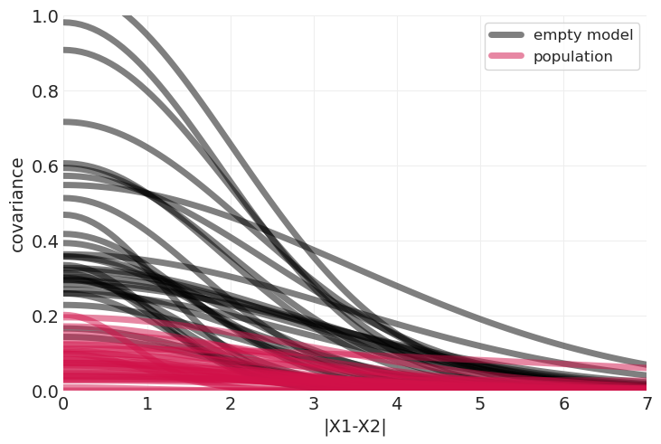
plot_predictive_covariance(distance_inference.posterior, color="k", label="empty model")
plot_predictive_covariance(distance_population_inference.posterior, label="population")
plt.ylim([0, 1]);

distance_population_model_covariance = calculate_posterior_mean_covariance_matrix(
    distance_population_inference
)
plot_posterior_mean_covariance_matrix(distance_population_model_covariance)

Posterior Mean Kernel parameters:
eta_squared: 0.1545764701828998
rho_squared: 0.19242529419650606

我们可以看到，通过包含人口，与仅距离模型相比，解释工具使用所需的协方差程度降低了。即，人口已经解释了更多的变异。

plot_kline_model_covarance(distance_population_model_covariance, max_cov=0.4)
plt.title("Stratifying by Population");

拟合仅人口模型以进行比较

我认为这就是 McElreath 构建图表的方式，该图表结合了人口规模、工具使用和岛屿协方差（下图）。具体来说，我们使用解析解估计仅人口模型，但不包括岛屿之间的协方差。然后，我们在该模型之上添加协方差图，以证明即使在模型中包含人口的情况下，关于协方差仍然有一些信息被遗漏。

ETA = 5.1  # Exponential hyperparmeter taken from Lecture 10 notes
with pm.Model() as population_model:

    # Note: raw population here, not log/standardized
    population = pm.Data("population", KLINE.logpop.values)

    # Priors
    # innovation rate
    alpha = pm.Exponential("alpha", eta)

    # Contact-level elasticity
    beta = pm.Exponential("beta", eta)

    # G lobal technology loss rate
    gamma = pm.Exponential("gamma", eta)

    # Likelihood using difference equation equilibrium as mean Poisson rate
    lamb = (alpha * (population**beta)) / gamma
    pm.Poisson("tools", lamb, observed=TOOLS)

    population_inference = pm.sample(tune=2000, target_accept=0.98)
    population_inference = pm.sample_posterior_predictive(
        population_inference, extend_inferencedata=True
    )

Initializing NUTS using jitter+adapt_diag...
Multiprocess sampling (4 chains in 4 jobs)
NUTS: [alpha, beta, gamma]

Sampling 4 chains for 2_000 tune and 1_000 draw iterations (8_000 + 4_000 draws total) took 10 seconds.
Sampling: [tools]

def plot_kline_model_population_covariance(
    covariance_matric, min_alpha=0.01, alpha_gain=1, max_cov=None
):

    # Plot covariancef
    max_cov = covariance_matric.max() if max_cov is None else max_cov
    for ii in range(10):
        for jj in range(10):
            if ii != jj:
                logpop_a = KLINE.loc[ii, "logpop"]
                tools_a = KLINE.loc[ii, "total_tools"]

                logpop_b = KLINE.loc[jj, "logpop"]
                tools_b = KLINE.loc[jj, "total_tools"]
                cov = covariance_matric[ii, jj]
                alpha = (min_alpha + (1 - min_alpha) * (cov / max_cov)) ** (1 / alpha_gain)
                plt.plot(
                    (logpop_a, logpop_b), (tools_a, tools_b), linewidth=3, color="k", alpha=alpha
                )

    plt.scatter(KLINE.logpop, KLINE.total_tools, s=KLINE.population * 0.01, zorder=10)

    # Annotate
    for ii in range(10):
        plt.annotate(
            KLINE.loc[ii, "culture"],
            (KLINE.loc[ii, "logpop"] + 0.1, KLINE.loc[ii, "total_tools"]),
            zorder=11,
            color="C1",
            fontsize=12,
            fontweight="bold",
        )
    plt.xlabel("log population")
    plt.ylabel("total tools")
    plt.axis("tight")


def plot_kline_population_only_model_posterior_predictive(inference):
    ppd = inference.posterior_predictive["tools"]
    az.plot_hdi(
        x=KLINE.logpop,
        y=ppd,
        color="C1",
        hdi_prob=0.89,
        fill_kwargs={"alpha": 0.1},
    )

    plt.plot(
        KLINE.logpop,
        ppd.mean(dim=("chain", "draw")),
        color="C1",
        linewidth=4,
        alpha=0.5,
        label="Population-only Model",
    )
    plt.legend()


plot_kline_model_population_covariance(distance_population_model_covariance, max_cov=0.4)
plot_kline_population_only_model_posterior_predictive(population_inference)

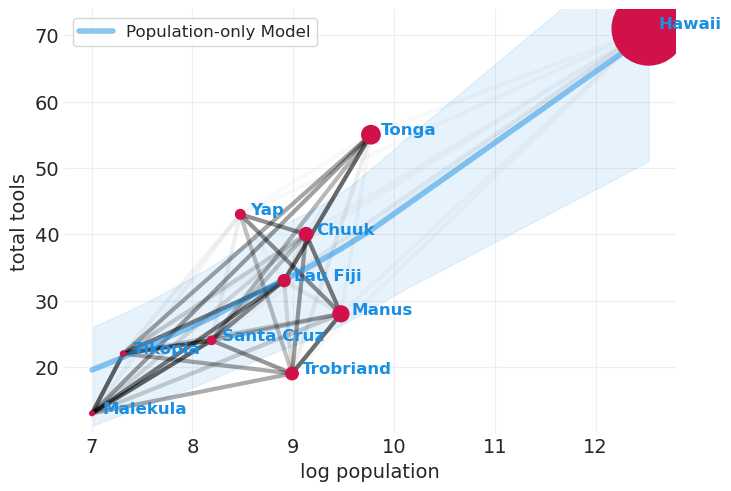
虽然仅人口就解释了工具使用中的大部分方差（蓝色曲线），但仍然存在相当多的残余岛屿-岛屿相似性可以解释工具使用（即，一些黑线仍然具有一定的权重）。

系统发育回归

数据集：Primates301

PRIMATES301 = utils.load_data("Primates301")
PRIMATES301.head()

	名称	属	物种	亚种	spp_id	genus_id	社会学习	研究投入	大脑	身体	群体大小	妊娠期	断奶	寿命	性成熟	母体投入
0	Allenopithecus_nigroviridis	Allenopithecus	nigroviridis	NaN	1	1	0.0	6.0	58.02	4655.00	40.0	NaN	106.15	276.0	NaN	NaN
1	Allocebus_trichotis	Allocebus	trichotis	NaN	2	2	0.0	6.0	NaN	78.09	1.0	NaN	NaN	NaN	NaN	NaN
2	Alouatta_belzebul	Alouatta	belzebul	NaN	3	3	0.0	15.0	52.84	6395.00	7.4	NaN	NaN	NaN	NaN	NaN
3	Alouatta_caraya	Alouatta	caraya	NaN	4	3	0.0	45.0	52.63	5383.00	8.9	185.92	323.16	243.6	1276.72	509.08
4	Alouatta_guariba	Alouatta	guariba	NaN	5	3	0.0	37.0	51.70	5175.00	7.4	NaN	NaN	NaN	NaN	NaN

• 301 种灵长类物种

• 生活史特征

• 体重 \(M\)，大脑大小 \(B\)，社会群体大小 \(G\)

• 测量误差，未观察到的混淆

• 缺失数据，我们将在本次讲座中重点关注完整案例分析

筛选出 151 个完整案例

删除缺失体重、大脑大小或群体大小的观测值

PRIMATES = PRIMATES301.query(
    "brain.notnull() and body.notnull() and group_size.notnull()", engine="python"
)
PRIMATES

	名称	属	物种	亚种	spp_id	genus_id	社会学习	研究投入	大脑	身体	群体大小	妊娠期	断奶	寿命	性成熟	母体投入
0	Allenopithecus_nigroviridis	Allenopithecus	nigroviridis	NaN	1	1	0.0	6.0	58.02	4655.0	40.00	NaN	106.15	276.0	NaN	NaN
2	Alouatta_belzebul	Alouatta	belzebul	NaN	3	3	0.0	15.0	52.84	6395.0	7.40	NaN	NaN	NaN	NaN	NaN
3	Alouatta_caraya	Alouatta	caraya	NaN	4	3	0.0	45.0	52.63	5383.0	8.90	185.92	323.16	243.6	1276.72	509.08
4	Alouatta_guariba	Alouatta	guariba	NaN	5	3	0.0	37.0	51.70	5175.0	7.40	NaN	NaN	NaN	NaN	NaN
5	Alouatta_palliata	Alouatta	palliata	NaN	6	3	3.0	79.0	49.88	6250.0	13.10	185.42	495.60	300.0	1578.42	681.02
...	...	...	...	...	...	...	...	...	...	...	...	...	...	...	...	...
294	Trachypithecus_obscurus	Trachypithecus	obscurus	NaN	295	67	0.0	6.0	62.12	7056.0	10.00	146.63	362.93	300.0	NaN	509.56
295	Trachypithecus_phayrei	Trachypithecus	phayrei	NaN	296	67	0.0	16.0	72.84	7475.0	12.90	180.61	305.87	NaN	NaN	486.48
296	Trachypithecus_pileatus	Trachypithecus	pileatus	NaN	297	67	0.0	5.0	103.64	11794.0	8.50	NaN	NaN	NaN	NaN	NaN
298	Trachypithecus_vetulus	Trachypithecus	vetulus	NaN	299	67	0.0	2.0	61.29	6237.0	8.35	204.72	245.78	276.0	1113.70	450.50
300	Varecia_variegata_variegata	Varecia	variegata	variegata	301	68	0.0	57.0	32.12	3575.0	2.80	102.50	90.73	384.0	701.52	193.23

151 行 × 16 列

变量之间存在大量协变

from seaborn import pairplot

pairplot(
    PRIMATES.assign(
        log_brain_volume=lambda x: np.log(x["brain"]),
        log_body_mass=lambda x: np.log(x["body"]),
        log_group_size=lambda x: np.log(x["group_size"]),
    )[["log_brain_volume", "log_body_mass", "log_group_size"]]
);

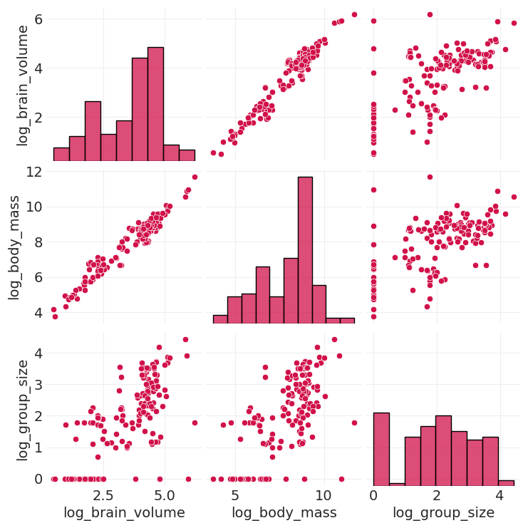
仅从样本中无法知道是什么导致了什么

因果沙拉

• 将所有预测变量投入模型，然后因果地解释它们的系数

• 使用预测方法作为因果关系的替代

• 将所有因素投入到回归项的“沙拉”中

  • 基于预测执行模型选择（我们在第 07 讲 - 过拟合和欠拟合中展示了为什么这样做不好）

  • 并将结果系数解释为因果效应（我们已经多次展示了为什么这样做不好）

• 控制系统发育很重要，但通常是在不经思考的情况下完成的（使用“沙拉”方法）

• 具有系统发育的回归仍然需要因果模型

不同的假设需要不同的因果模型 (DAG)

社会大脑假说

• 群体大小 \(G\) 影响大脑大小 \(B\)

体重 \(M\) 是 \(M\) 和 \(B\) 的共同原因

这是我们将在本次讲座中重点关注的 DAG

utils.draw_causal_graph(edge_list=[("G", "B"), ("M", "G"), ("M", "B")], graph_direction="LR")

体重 \(M\) 是 \(M\) 和 \(B\) 的中介

utils.draw_causal_graph(edge_list=[("G", "B"), ("G", "M"), ("M", "B")], graph_direction="LR")

大脑大小 \(B\) 实际上导致群体大小 \(G\)；\(M\) 仍然是两者的共同原因

utils.draw_causal_graph(edge_list=[("B", "G"), ("M", "G"), ("M", "B")], graph_direction="LR")

未观察到的混淆因素使对特征进行朴素回归而不控制历史变得危险

• 历史会引入许多未观察到的共享混淆因素，我们需要尝试控制这些因素。

• 系统发育历史可以作为这些共享混淆因素的代理。

• 我们只有当前对历史结果的测量

  • 实际的系统发育不存在

  • 基因组的不同部分可以有不同的历史

但是，假设我们确实有一个推断的系统发育（正如我们在本次讲座中所做的那样），我们使用此系统发育，结合高斯过程回归，将物种之间的相似性建模为共享历史的代理

utils.draw_causal_graph(
    edge_list=[("G", "B"), ("M", "G"), ("M", "B"), ("u", "M"), ("u", "G"), ("u", "B"), ("h", "u")],
    node_props={
        "h": {"label": "history\n(phylogeny)"},
        "u": {"style": "dashed", "label": "confounds, u"},
        "unobserved": {"style": "dashed"},
    },
    graph_direction="LR",
)

系统发育回归

• 遗传进化历史悠久

• 我们只能测量该过程的当前最终状态

• 原则上，共同的遗传历史应该会引起物种之间的协变

• 我们应该能够对这种协变进行建模，以平均所有可能导致遗传相似性（宏观状态）的历史（微观状态）

两个共同的问题

1. 什么是历史（系统发育）？

2. 我们如何使用它来建模原因和控制混淆因素？

1. 什么是历史（系统发育）？

我们如何估计或识别系统发育？

困难

• 高度不确定性

• 过程是非平稳的

  • 基因组的不同部分具有不同的历史

  • 交叉效应

• 可用的推断工具

  • 探索树空间很困难

  • 将其他领域的软件重新用于研究生物学

• 系统发育（就像社交网络一样）不存在。

  • 它们是我们用来捕捉数据规律性的抽象概念

2. 我们如何使用它来建模原因？

……假设我们已经获得了系统发育，现在怎么办？

方法

• 没有默认方法

• 高斯过程是默认方法

  • 使用系统发育作为“遗传距离”的代理

线性回归的两种等效公式

您始终可以使用来自多元正态分布的抽样重新表达线性回归

经典线性回归

数据集 \(\textbf{B}\) 被建模为来自随机单变量正态分布的 \(D\) 个独立样本 \(B_i\)。$$

()\[\begin{align} B_i &\sim \text{Normal}(\mu_i, \sigma^2) \\ \mu_i &= \alpha + \beta_G G_i + \beta_M M_i \\ \alpha &\sim \text{Normal}(0, 1) \\ \beta_{G, M} &\sim \text{Normal}(0, 1) \\ \sigma &\sim \text{Exponential}(1) \end{align}\]

\[### $\text{MVNormal}$ 公式 数据集被建模为从 $\text{MVNormal}$ 采样的单个 $D$-向量 $\textbf{B}$。更具有高斯过程的味道；允许我们制定线性回归，以便包含输出之间的协变。\]

()\[\begin{align} \textbf{B} &\sim \text{MVNormal}(\mu, \textbf{K}) \\ \mathbf{K} &= \mathbf{I}\sigma^2 \\ \mu_i &= \alpha + \beta_G G_i + \beta_M M_i \\ \alpha &\sim \text{Normal}(0, 1) \\ \beta_{G, M} &\sim \text{Normal}(0, 1) \\ \sigma &\sim \text{Exponential}(1) \end{align}\]

$$

经典线性回归

# Preprocessing used in the Lecture
G = utils.standardize(np.log(PRIMATES.group_size.values))
M = utils.standardize(np.log(PRIMATES.body.values))
B = utils.standardize(np.log(PRIMATES.brain.values))

with pm.Model() as vanilla_lr_model:
    # Priors
    alpha = pm.Normal("alpha", 0, 1)
    beta_G = pm.Normal("beta_G", 0, 0.5)
    beta_M = pm.Normal("beta_M", 0, 0.5)
    sigma = pm.Exponential("sigma", 1)

    # Likelihood
    mu = alpha + beta_G * G + beta_M * M
    pm.Normal("B", mu=mu, sigma=sigma, observed=B)

    vanilla_lr_inference = pm.sample()

Initializing NUTS using jitter+adapt_diag...
Multiprocess sampling (4 chains in 4 jobs)
NUTS: [alpha, beta_G, beta_M, sigma]

Sampling 4 chains for 1_000 tune and 1_000 draw iterations (4_000 + 4_000 draws total) took 1 seconds.

\(\text{MVNormal}\) 线性回归

with pm.Model() as vector_lr_model:

    # Priors
    alpha = pm.Normal("alpha", 0, 1)
    beta_G = pm.Normal("beta_G", 0, 0.5)
    beta_M = pm.Normal("beta_M", 0, 0.5)
    sigma = pm.Exponential("sigma", 1)

    # Likelihood
    K = np.eye(len(B)) * sigma**2
    mu = alpha + beta_G * G + beta_M * M
    pm.MvNormal("B", mu=mu, cov=K, observed=B)

    vector_lr_inference = pm.sample()

Initializing NUTS using jitter+adapt_diag...
Multiprocess sampling (4 chains in 4 jobs)
NUTS: [alpha, beta_G, beta_M, sigma]

Sampling 4 chains for 1_000 tune and 1_000 draw iterations (4_000 + 4_000 draws total) took 18 seconds.

验证这两个公式是否提供相同的参数估计

我们能够恢复与讲座中相同的估计值

pm.summary(vanilla_lr_inference, round_to=2)

	均值	标准差	hdi_3%	hdi_97%	mcse_mean	mcse_sd	ess_bulk	ess_tail	r_hat
alpha	-0.00	0.02	-0.03	0.03	0.0	0.0	3539.69	3113.60	1.0
beta_G	0.12	0.02	0.08	0.17	0.0	0.0	2677.36	3066.65	1.0
beta_M	0.89	0.02	0.85	0.94	0.0	0.0	2753.50	2995.51	1.0
sigma	0.22	0.01	0.20	0.24	0.0	0.0	3669.05	2850.15	1.0

pm.summary(vector_lr_inference, round_to=2)

	均值	标准差	hdi_3%	hdi_97%	mcse_mean	mcse_sd	ess_bulk	ess_tail	r_hat
alpha	0.00	0.02	-0.03	0.03	0.0	0.0	3738.52	3261.00	1.0
beta_G	0.12	0.02	0.08	0.17	0.0	0.0	2972.04	2931.39	1.0
beta_M	0.89	0.02	0.85	0.94	0.0	0.0	2958.08	2856.22	1.0
sigma	0.22	0.01	0.19	0.24	0.0	0.0	3697.40	2635.74	1.0

从模型到核

我们想将一些残差 \(u_i\) 纳入我们的线性回归中，以调整期望值，从而编码物种的共同历史

\[\begin{split} \begin{align} \textbf{B} &\sim \text{MVNormal}(\mu, \textbf{K}) \\ \mathbf{K} &= \mathbf{I}\sigma^2 \\ \mu_i &= \alpha + \beta_G G_i + \beta_M M_i + u_i\\ \alpha &\sim \text{Normal}(0, 1) \\ \beta_{G, M} &\sim \text{Normal}(0, 1) \\ \sigma &\sim \text{Exponential}(1) \end{align} \end{split}\]

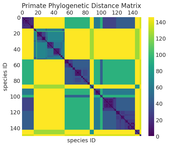
系统发育距离作为物种协方差的代理

• 协方差随系统发育距离衰减

  • 树中叶节点之间的路径长度（例如，参见下面的树状图）

• 可以像我们在海洋工具分析中对岛屿距离所做的那样，以非常相似的方式使用高斯过程

PRIMATES_DISTANCE_MATRIX301 = utils.load_data("Primates301_distance_matrix").values
# Filter out incomplete cases
PRIMATES_DISTANCE_MATRIX = PRIMATES_DISTANCE_MATRIX301[PRIMATES.index][:, PRIMATES.index]

fig, ax = plt.subplots(figsize=(6, 5))
im = ax.matshow(PRIMATES_DISTANCE_MATRIX)
ax.grid(None)
fig.colorbar(im, orientation="vertical")
plt.xlabel("species ID")
plt.ylabel("species ID")
ax.set_title("Primate Phylogenetic Distance Matrix");

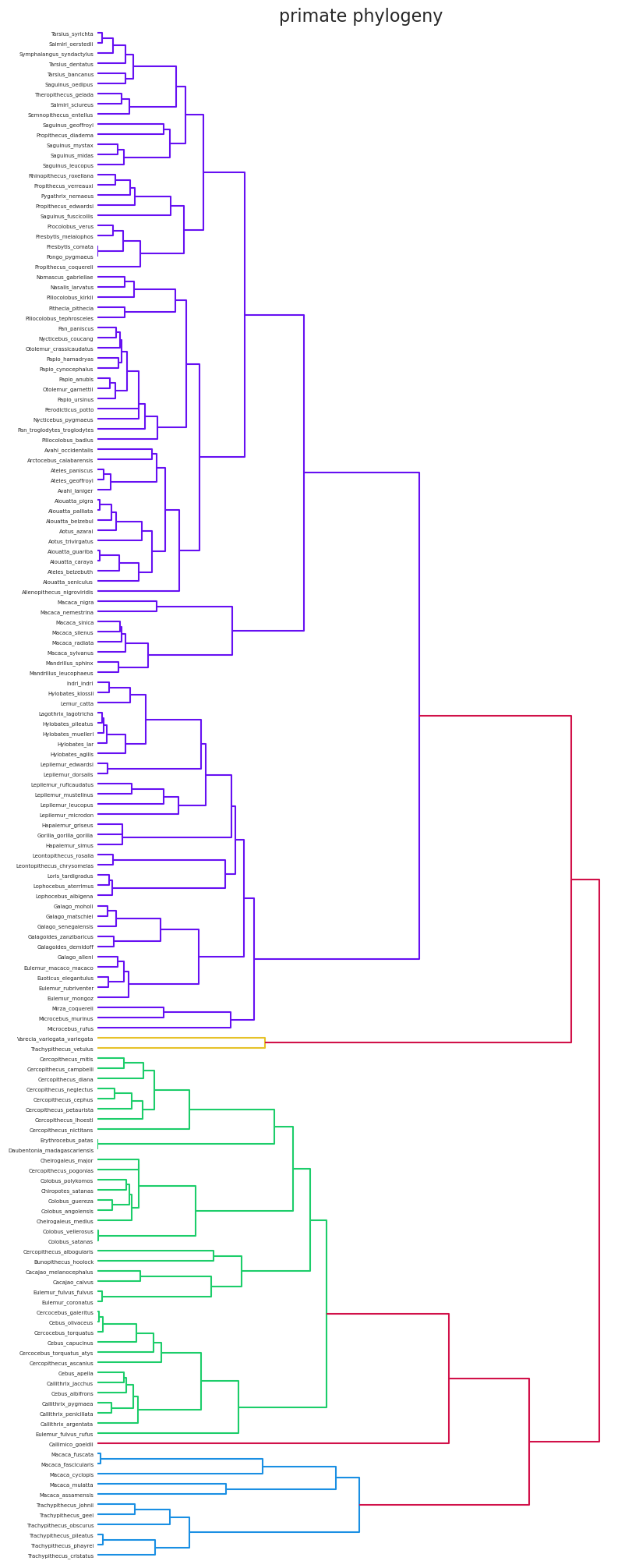
# Plot the distance matrix
from scipy.cluster.hierarchy import dendrogram, linkage
from scipy.spatial.distance import squareform

dists = squareform(PRIMATES_DISTANCE_MATRIX)
linkage_matrix = linkage(dists, "single")
plt.subplots(figsize=(8, 20))
dendrogram(linkage_matrix, orientation="right", distance_sort=True, labels=PRIMATES.name.tolist())
plt.title("primate phylogeny")
plt.grid(False)
plt.xticks([]);

核函数作为进化动态的代理

def brownian_motion_kernel(X0, X1, a=1, c=1):
    k = 1 / a * ((X0 - c) @ (X1 - c).T)[::-1, ::-1]
    return k


plt.subplots(figsize=(5, 5))
plot_kernel_function(
    partial(brownian_motion_kernel, a=22000), max_distance=150, label='Linear\n"Brownian Motion"'
)
plot_kernel_function(
    partial(ornstein_uhlenbeck_kernel, rho=1 / 20),
    max_distance=150,
    color="C1",
    label='Ornstein-Uhlenbeck\n"Damped Brownian Motion"',
)
plt.xlabel("phylogenetic distance");

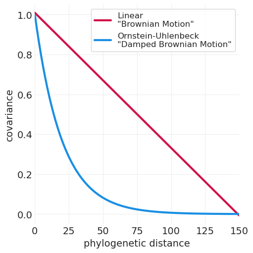
进化模型 + 树结构 = 在末梢观察到的协变模式

常见的简单进化动态模型

• 布朗运动 - 意味着线性协方差核函数

• 阻尼布朗运动 - 意味着 L1 / 奥恩斯坦-乌伦贝克协方差核函数

系统发育“回归”模型

\[\begin{split} \begin{align} \textbf{B} &\sim \text{MVNormal}(\mu, \textbf{K}) \\ \mathbf{K} &= \eta^2 \exp(-\rho D_{ij}) &\text{奥恩斯坦-乌伦贝克核}\\ \mu_i &= \alpha + \beta_G G_i + \beta_M M_i \\ \alpha &\sim \text{Normal}(0, 1) \\ \beta_{G, M} &\sim \text{Normal}(0, 1) \\ \eta^2 &\sim \text{HalfNormal}(1, 0.25) &\text{最大协方差先验} \\ \rho &\sim \text{HalfNormal}(3, 0.25) &\text{协方差衰减率先验} \end{align} \end{split}\]

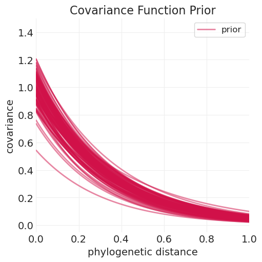
奥恩斯坦-乌伦贝克核模型的先验样本

eta_squared_samples = pm.draw(pm.TruncatedNormal.dist(mu=1, sigma=0.25, lower=0.01), 100) ** 0.5
rho_samples = pm.draw(pm.TruncatedNormal.dist(mu=3, sigma=0.25, lower=0.01), 100)

plt.subplots(figsize=(5, 5))
for ii, (eta_squared_, rho_) in enumerate(zip(eta_squared_samples, rho_samples)):
    label = "prior" if ii == 0 else None
    kernel_function = partial(ornstein_uhlenbeck_kernel, eta_squared=eta_squared_, rho=rho_)
    plot_kernel_function(
        kernel_function, color="C0", label=label, alpha=0.5, linewidth=2, max_distance=1
    )

plt.ylim([-0.05, 1.5])
plt.xlabel("phylogenetic distance")
plt.ylabel("covariance")
plt.title("Covariance Function Prior");

仅距离模型

• 使高斯过程部分工作，然后添加细节

• 设置 \(\beta_M = \beta_G = 0\)

# Rescale distances from 0 to 1
D = PRIMATES_DISTANCE_MATRIX / PRIMATES_DISTANCE_MATRIX.max()
assert D.max() == 1

PyMC 实现

以下是使用 PyMC 高斯过程模块的实现。

• 在上面的海洋工具模型中，我们不需要高斯过程具有均值函数，因为所有变量都已标准化，因此我们可以使用默认均值函数 \(0\)

• 对于系统发育回归，我们不再需要零均值函数，但我们需要均值函数依赖于 \(M\) 和 \(G\)，而不是系统发育距离矩阵的函数。我们可以在 pymc 中实现自定义均值函数来处理这个问题

• 此外，由于我们的似然函数是 MVNormal，我们可以利用 GP 先验和正态似然之间的共轭性，这将返回 GP 后验。这意味着我们应该使用 pm.gp.Marginal 而不是 pm.gp.Latent，后者使用后验的闭式解来加速学习。

class MeanBodyMassSocialGroupSize(pm.gp.mean.Linear):
    """Custom mean function that separates covariates from phylogeny"""

    def __init__(self, alpha, beta_G, beta_M):
        self.alpha = alpha
        self.beta_G = beta_G
        self.beta_M = beta_M

    def __call__(self, X):
        return self.alpha + self.beta_G * G + self.beta_M * M

PRIMATE_ID, PRIMATE = pd.factorize(PRIMATES["name"], sort=False)
with pm.Model(coords={"primate": PRIMATE}) as intercept_only_phylogenetic_mvn_model:
    # Priors
    alpha = pm.Normal("alpha", 0, 1)
    sigma = pm.Exponential("sigma", 1)

    # Intercept-only model
    beta_M = 0
    beta_G = 0

    # Define the mean function
    mean_func = MeanBodyMassSocialGroupSize(alpha, beta_G, beta_M)

    # Phylogenetic distance covariance
    eta_squared = pm.TruncatedNormal("eta_squared", 1, 0.25, lower=0.01)
    rho = pm.TruncatedNormal("rho", 3, 0.25, lower=0.01)

    # For Ornstein-Uhlenbeck kernel we can use Matern 1/2 or Exponential covariance Function
    cov_func = eta_squared * pm.gp.cov.Matern12(1, ls=rho)
    # cov_func = eta_squared * pm.gp.cov.Exponential(1, ls=rho)

    # Init the GP
    gp = pm.gp.Marginal(mean_func=mean_func, cov_func=cov_func)

    # Likelihood
    gp.marginal_likelihood("B", X=D, y=B, noise=sigma)
    intercept_only_phylogenetic_mvn_inference = pm.sample(target_accept=0.9)

Initializing NUTS using jitter+adapt_diag...
Multiprocess sampling (4 chains in 4 jobs)
NUTS: [alpha, sigma, eta_squared, rho]

Sampling 4 chains for 1_000 tune and 1_000 draw iterations (4_000 + 4_000 draws total) took 30 seconds.

以下是另一种实现方式，它手动构建协方差函数，并直接将数据集建模为具有均值 alpha 和由核定义的协方差的 MVNormal。我发现这些直接的 MVNormal 实现与讲座的思路更一致

def generate_L1_kernel_matrix(D, eta_squared, rho, smoothing=0.1):
    K = eta_squared * pm.math.exp(-rho * D)

    # Smooth the diagonal of the covariance matrix
    N = D.shape[0]
    K += np.eye(N) * smoothing
    return K


# with pm.Model() as intercept_only_phylogenetic_mvn_model:

#     # Priors
#     alpha = pm.Normal("alpha", 0, 1)

#     # Phylogenetic distance covariance
#     eta_squared = pm.TruncatedNormal("eta_squared", 1, 0.25, lower=.001)
#     rho = pm.TruncatedNormal("rho", 3, 0.25, lower=.001)

#     # Ornstein-Uhlenbeck kernel
#     K = pm.Deterministic('K', generate_L1_kernel_matrix(D, eta_squared, rho))
#     # K = pm.Deterministic('K', eta_squared * pm.math.exp(-rho * D))

#     # Likelihood
#     mu = pm.math.ones_like(B) * alpha
#     pm.MvNormal("B", mu=mu, cov=K, observed=B)
#     intercept_only_phylogenetic_mvn_inference = pm.sample(target_accept=.98)

az.summary(intercept_only_phylogenetic_mvn_inference, var_names=["alpha", "eta_squared", "rho"])

	均值	标准差	hdi_3%	hdi_97%	mcse_mean	mcse_sd	ess_bulk	ess_tail	r_hat
alpha	0.080	0.704	-1.279	1.355	0.011	0.011	3952.0	2810.0	1.0
eta_squared	1.063	0.236	0.633	1.519	0.005	0.003	2611.0	1753.0	1.0
rho	2.973	0.251	2.510	3.448	0.004	0.003	4027.0	2757.0	1.0

# Sample the prior for comparison
with intercept_only_phylogenetic_mvn_model:
    intercept_only_phylogenetic_mvn_prior = pm.sample_prior_predictive().prior

az.summary(intercept_only_phylogenetic_mvn_prior, var_names=["alpha", "eta_squared", "rho"])

Sampling: [B, alpha, eta_squared, rho, sigma]
arviz - WARNING - Shape validation failed: input_shape: (1, 500), minimum_shape: (chains=2, draws=4)

	均值	标准差	hdi_3%	hdi_97%	mcse_mean	mcse_sd	ess_bulk	ess_tail	r_hat
alpha	-0.053	0.984	-1.989	1.755	0.045	0.032	484.0	412.0	NaN
eta_squared	1.001	0.254	0.548	1.463	0.012	0.009	444.0	339.0	NaN
rho	3.014	0.247	2.541	3.431	0.011	0.008	465.0	447.0	NaN

比较仅距离模型的先验和后验

def calculate_mean_covariance_matrix(inference):
    def distance_to_covariance(distance, eta_squared, rho):
        return eta_squared * np.exp(-rho * np.abs(distance))

    inference_mean = inference.mean(dim=("chain", "draw"))

    eta_squared = inference_mean["eta_squared"].values
    rho = inference_mean["rho"].values

    print("Mean Kernel parameters:")
    print("eta_squared:", eta_squared)
    print("rho:", rho)

    n_species = D.shape[0]
    model_covariance = np.zeros_like(D).astype(float)
    for ii in range(n_species):
        for jj in range(n_species):
            model_covariance[ii, jj] = distance_to_covariance(
                D[ii, jj], eta_squared=eta_squared, rho=rho
            )
    return model_covariance


def plot_mean_covariance_matrix(inference, title=None, max_cov=1.0):
    mean_cov = calculate_mean_covariance_matrix(inference)

    plt.imshow(mean_cov)
    # plt.imshow(inference['K'].mean(dim=('chain', 'draw')).values)
    plt.grid(None)
    plt.clim((0, max_cov))
    plt.colorbar()
    plt.xlabel("species ID")
    plt.ylabel("species ID")
    plt.title(title)

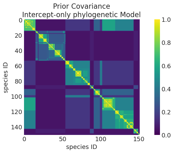
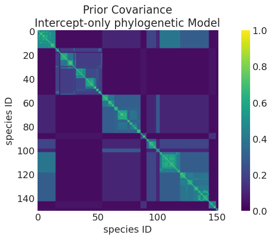
# Prior
plot_mean_covariance_matrix(
    intercept_only_phylogenetic_mvn_prior,
    title="Prior Covariance\nIntercept-only phylogenetic Model",
)

Mean Kernel parameters:
eta_squared: 1.0006788360203365
rho: 3.0138977110438527

# Posterior
plot_mean_covariance_matrix(
    intercept_only_phylogenetic_mvn_inference.posterior,
    title="Prior Covariance\nIntercept-only phylogenetic Model",
)

Mean Kernel parameters:
eta_squared: 1.062638229865811
rho: 2.9733158548987166

比较先验和后验核函数

def plot_predictive_kernel_function(predictive, n_samples=200, color="C0", label=None):

    eta_squared_samples = predictive["eta_squared"].values[0, :n_samples]
    rho_samples = predictive["rho"].values[0, :n_samples]

    for ii, (eta_squared_, rho_) in enumerate(zip(eta_squared_samples, rho_samples)):
        label = label if ii == 0 else None

        kernel_function = partial(ornstein_uhlenbeck_kernel, eta_squared=eta_squared_, rho=rho_)
        plot_kernel_function(
            kernel_function, color=color, label=label, alpha=0.1, linewidth=2, max_distance=1
        )

    plt.ylim([-0.05, 2.5])
    plt.xlabel("phylogenetic distance")

plot_predictive_kernel_function(intercept_only_phylogenetic_mvn_prior, label="prior", color="k")
plot_predictive_kernel_function(
    intercept_only_phylogenetic_mvn_inference.posterior, label="posterior B", color="C1"
)

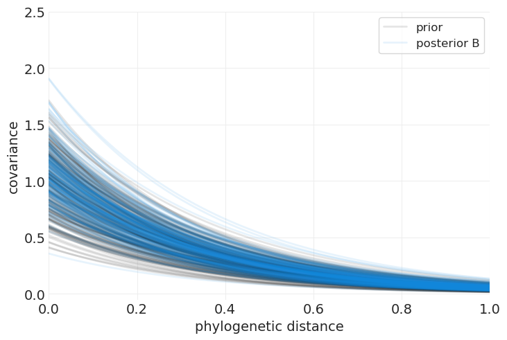
我们可以看到，通过比较核函数的先验和后验分布，模型已经从数据中学习，并减弱了我们对最大协方差的期望。

拟合完整的系统发育模型。

此模型按群体大小 \(G\) 和体重 \(M\) 分层

以下是使用 PyMC 高斯过程模块的实现。

with pm.Model(coords=coords) as full_phylogenetic_mvn_model:

    # Priors
    alpha = pm.Normal("alpha", 0, 1)
    sigma = pm.Exponential("sigma", 1)

    # Intercept-only model
    beta_M = pm.Normal("beta_M", 0, 1)
    beta_G = pm.Normal("beta_G", 0, 1)

    # Define the mean function
    mean_func = MeanBodyMassSocialGroupSize(alpha, beta_G, beta_M)

    # Phylogenetic distance covariance
    eta_squared = pm.TruncatedNormal("eta_squared", 1, 0.25, lower=0.01)
    rho = pm.TruncatedNormal("rho", 3, 0.25, lower=0.01)

    # For Ornstein-Uhlenbeck kernel we can use Matern 1/2 or Exponential covariance Function
    cov_func = eta_squared * pm.gp.cov.Matern12(1, ls=rho)
    # cov_func = eta_squared * pm.gp.cov.Exponential(1, ls=rho)

    # Init the GP
    gp = pm.gp.Marginal(mean_func=mean_func, cov_func=cov_func)

    # Likelihood
    gp.marginal_likelihood("B", X=D, y=B, noise=sigma)
    full_phylogenetic_mvn_inference = pm.sample(target_accept=0.9)

Initializing NUTS using jitter+adapt_diag...
Multiprocess sampling (4 chains in 4 jobs)
NUTS: [alpha, sigma, beta_M, beta_G, eta_squared, rho]

Sampling 4 chains for 1_000 tune and 1_000 draw iterations (4_000 + 4_000 draws total) took 53 seconds.
There were 7 divergences after tuning. Increase `target_accept` or reparameterize.
The rhat statistic is larger than 1.01 for some parameters. This indicates problems during sampling. See https://arxiv.org/abs/1903.08008 for details

以下是另一种实现方式，它手动构建协方差函数，并直接将数据集建模为 MVNormal，其均值是 \(G\) 和 \(M\) 的线性函数，协方差由核定义。我发现这些 MVNormal 实现与讲座的思路更一致。

# with pm.Model() as full_phylogenetic_mvn_model:

#     # Priors
#     alpha = pm.Normal("alpha", 0, 1)
#     beta_G = pm.Normal("beta_G", 0, 0.5)
#     beta_M = pm.Normal("beta_M", 0, 0.5)

#     # Phylogenetic distance covariance
#     eta_squared = pm.TruncatedNormal("eta_squared", 1, .25, lower=.001)
#     rho = pm.TruncatedNormal("rho", 3, .25, lower=.001)
#     K = pm.Deterministic('K', generate_L1_kernel_matrix(D, eta_squared, rho))
#     # K = pm.Deterministic('K', eta_squared * pm.math.exp(-rho * D))

#     mu = alpha + beta_G * G + beta_M * M

#     # Likelihood
#     pm.MvNormal("B", mu=mu, cov=K, observed=B)
#     full_phylogenetic_mvn_inference = pm.sample(target_accept=.98)

az.summary(
    full_phylogenetic_mvn_inference, var_names=["alpha", "eta_squared", "rho", "beta_M", "beta_G"]
)

	均值	标准差	hdi_3%	hdi_97%	mcse_mean	mcse_sd	ess_bulk	ess_tail	r_hat
alpha	-0.002	0.630	-1.197	1.194	0.011	0.011	3395.0	1985.0	1.00
eta_squared	0.726	0.318	0.015	1.199	0.010	0.007	972.0	471.0	1.01
rho	3.051	0.249	2.601	3.518	0.004	0.003	4011.0	2389.0	1.00
beta_M	0.901	0.023	0.858	0.942	0.000	0.000	2733.0	2739.0	1.00
beta_G	0.108	0.024	0.065	0.156	0.000	0.000	2669.0	2849.0	1.00

比较仅距离模型和完整系统发育回归模型中的协方差项

# Posterior
plot_mean_covariance_matrix(
    full_phylogenetic_mvn_inference.posterior,
    title="Prior Covariance\nIntercept-only phylogenetic Model",
)

Mean Kernel parameters:
eta_squared: 0.7258975020904833
rho: 3.0511929927563934

plot_predictive_kernel_function(intercept_only_phylogenetic_mvn_prior, label="prior", color="k")
plot_predictive_kernel_function(
    intercept_only_phylogenetic_mvn_inference.posterior, label="posterior B", color="C1"
)
plot_predictive_kernel_function(full_phylogenetic_mvn_inference.posterior, label="posterior BMG")

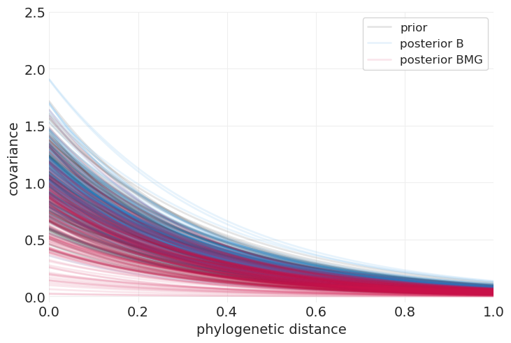
我们可以看到，当包含体重和群体大小的回归量时，与仅系统发育距离模型相比，用于解释大脑大小的系统发育协变量大大减少。

这里报告的完整系统发育模型的结果对我来说也很有意义，因为在控制了系统发育历史之后，我们可以主要通过体重来解释大脑大小的很多变异；这反过来使得系统发育历史在模型中获得较小的权重。

群体大小对大脑大小的影响

utils.draw_causal_graph(
    edge_list=[("G", "B"), ("M", "G"), ("M", "B"), ("u", "M"), ("u", "G"), ("u", "B"), ("h", "u")],
    node_props={
        "h": {"label": "history\n(phylogeny)", "color": "lightgray", "fontcolor": "lightgray"},
        "u": {
            "style": "dashed",
            "label": "confounds, u",
            "color": "lightgray",
            "fontcolor": "lightgray",
        },
        "unobserved": {"style": "dashed", "color": "lightgray", "fontcolor": "lightgray"},
    },
    edge_props={
        ("G", "B"): {"color": "blue"},
        ("M", "G"): {"color": "red"},
        ("M", "B"): {"color": "red"},
        ("u", "B"): {"color": "lightgray"},
        ("u", "M"): {"color": "lightgray"},
        ("u", "G"): {"color": "lightgray"},
        ("h", "u"): {
            "color": "lightgray",
        },
    },
    graph_direction="LR",
)

• 我们忽略了由于遗传历史造成的混淆因素（浅灰色）

  • 因此，我们不尝试控制由于遗传历史造成的潜在混淆因素。

• 为了获得 \(G\) 对 \(B\) 的直接影响，我们还将按 \(M\) 分层，以阻止通过经过 \(M\) 的叉路的后门路径。

with pm.Model() as ordinary_model:

    # Priors
    alpha = pm.Normal("alpha", 0, 1)
    beta_G = pm.Normal("beta_G", 0, 0.5)
    beta_M = pm.Normal("beta_M", 0, 0.5)

    # Independent species (equal variance)
    sigma = pm.Exponential("sigma", 1)
    K = np.eye(len(B)) * sigma

    mu = alpha + beta_G * G + beta_M * M

    pm.MvNormal("B", mu=mu, cov=K, observed=B)
    ordinary_inference = pm.sample()

Initializing NUTS using jitter+adapt_diag...
Multiprocess sampling (4 chains in 4 jobs)
NUTS: [alpha, beta_G, beta_M, sigma]

Sampling 4 chains for 1_000 tune and 1_000 draw iterations (4_000 + 4_000 draws total) took 18 seconds.

az.summary(ordinary_inference, var_names=["alpha", "beta_M", "beta_G"])

	均值	标准差	hdi_3%	hdi_97%	mcse_mean	mcse_sd	ess_bulk	ess_tail	r_hat
alpha	-0.000	0.018	-0.035	0.032	0.0	0.0	4259.0	2653.0	1.0
beta_M	0.892	0.023	0.850	0.936	0.0	0.0	3054.0	3040.0	1.0
beta_G	0.123	0.023	0.078	0.165	0.0	0.0	2941.0	2882.0	1.0

def plot_primate_posterior_comparison(variable, ax, title=None):
    az.plot_dist(ordinary_inference.posterior[variable], color="k", label="ordinary", ax=ax)
    az.plot_dist(
        full_phylogenetic_mvn_inference.posterior[variable],
        color="C0",
        label="Ornstein-Uhlenbeck",
        ax=ax,
    )
    ax.axvline(0, color="k", linestyle="--")
    ax.set_xlabel(f"$\\{variable}$")
    ax.set_ylabel("density")
    ax.set_title(title)


_, axs = plt.subplots(1, 2, figsize=(10, 5))
plot_primate_posterior_comparison("beta_G", axs[0], "Effect of Group Size\non Brain Size")
plot_primate_posterior_comparison("beta_M", axs[1], "Effect of Body Mass\non Brain size")

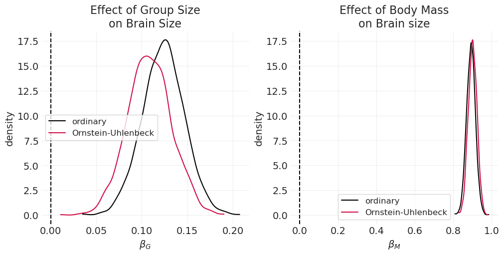
通过尝试控制由于遗传历史造成的潜在混淆因素，我们几乎将群体大小对大脑大小的估计影响 \(\beta_G\) 减半，尽管它仍然主要是正面的。

此估计器还可以为我们提供体重 \(M\) 对大脑大小 \(B\) 的直接影响（通过阻止通过 \(G\) 的管道）。当我们查看 \(\beta_M\) 时，我们看到当控制遗传历史混淆因素时，体重对大脑大小的影响略有增加，尽管对于两个估计器而言，这种影响都很大，表明体重是大脑大小的重要驱动因素。

总结：系统发育回归

潜在问题

• 系统发育的不确定性如何？

  • 最好同时执行系统发育推断——即估计系统发育的后验

• 互惠因果关系如何？

  • 生物体与环境之间的反馈

  • 不存在单向原因

  • 因此回归可能不是最佳选择

  • 新的方法包括微分方程，将问题表述为多目标优化问题

总结：高斯过程

• 为连续组/类别提供（局部）部分池化的方法

• 通用近似引擎 – 适用于预测

• 对过拟合稳健

• 对先验敏感：先验预测模拟非常重要

作者

• 由 Dustin Stansbury (2024) 移植到 PyMC

• 基于 Richard McElreath 的统计再思考 (2023) 讲座

%load_ext watermark
%watermark -n -u -v -iv -w -p pytensor,aeppl,xarray

Last updated: Tue Dec 17 2024

Python implementation: CPython
Python version       : 3.12.5
IPython version      : 8.27.0

pytensor: 2.26.4
aeppl   : not installed
xarray  : 2024.7.0

seaborn    : 0.13.2
scipy      : 1.14.1
matplotlib : 3.9.2
numpy      : 1.26.4
xarray     : 2024.7.0
statsmodels: 0.14.2
pymc       : 5.19.1
arviz      : 0.19.0
pandas     : 2.2.2

Watermark: 2.5.0

许可证声明

此示例库中的所有笔记本均根据 MIT 许可证提供，该许可证允许修改和再分发以用于任何用途，前提是保留版权和许可证声明。

引用 PyMC 示例

要引用此笔记本，请使用 Zenodo 为 pymc-examples 存储库提供的 DOI。

重要提示

许多笔记本改编自其他来源：博客、书籍…… 在这种情况下，您也应该引用原始来源。

另请记住引用您的代码使用的相关库。

这是一个 bibtex 中的引用模板

@incollection{citekey,
  author    = "<notebook authors, see above>",
  title     = "<notebook title>",
  editor    = "PyMC Team",
  booktitle = "PyMC examples",
  doi       = "10.5281/zenodo.5654871"
}

一旦呈现，它可能看起来像