测量与误分类

此笔记本是 PyMC 移植的 Statistical Rethinking 2023 Richard McElreath 讲座系列的一部分。

视频 - 第 17 讲 - 测量与误分类# 第 17 讲 - 测量与误分类

# Ignore warnings
import warnings

import arviz as az
import numpy as np
import pandas as pd
import pymc as pm
import pytensor.tensor as pt
import statsmodels.formula.api as smf
import utils as utils
import xarray as xr

from matplotlib import pyplot as plt
from matplotlib import style
from scipy import stats as stats

warnings.filterwarnings("ignore")

# Set matplotlib style
STYLE = "statistical-rethinking-2023.mplstyle"
style.use(STYLE)

概率、直觉和煎饼 🥞

McElreath 提出了对 经典蒙提霍尔问题 的重新阐述。 最初的问题使用一个名为“Let’s Make a Deal”（由 Monty Hall 主持）的旧游戏节目作为背景，描述了一个场景，在该场景中，赢得游戏的正确、最佳策略是通过遵循概率论规则给出的。 蒙提霍尔问题有趣的地方在于，最佳策略与我们的直觉不符。

在讲座中，我们不是像蒙提霍尔问题那样打开门寻找驴子或奖品，而是有煎饼，它们的两面要么是烤焦的，要么是完美烹制的。 思想实验是这样的

• 你有 3 个煎饼

  • 一个（很可能是你做的第一个）两面都烤焦了

  • 一个（很可能是你改进烹饪技巧后做的下一个）只有一面烤焦了

  • 一个是两面都完美烹制的

• 假设你随机得到一个煎饼，它的一面烤焦了

• 另一面烤焦的概率是多少？

大多数人会说 1/2，这直觉上感觉是正确的。 然而，正确答案由贝叶斯规则给出

如果我们定义 \(U, D\) 为观察到正面 \(U\) 或反面 \(D\) 未烤焦，\(U', D'\) 为正面或反面烤焦

\[\begin{split} \begin{align*} p(D' | U') &= \frac{p(U', D')}{p(U')} &\text{贝叶斯规则} \\ p(U', D') &= 1/3 &\text{三个煎饼中只有一个两面都烤焦了} \\ p(U') &= (1/3 \times 2/2) + (1/3 \times 1/2) + (1/3 \times 0) = 3/6 = 1/2 &\text{最初观察到正面烤焦的概率} \\ p(D' | U') &= \frac{1/3}{1/2} = 2/3 \end{align*} \end{split}\]

避免耍小聪明

• 耍小聪明是不可靠的

• 耍小聪明是不透明的

• 你很少能战胜概率论的公理

• 如果我们坚持规则，概率允许我们解决复杂的问题

测量误差

• 许多变量是我们想要测量的东西的代理（例如，后代基本混杂因素）

• 忽略测量误差是一种常见的做法

  • 假设误差是无害的，或者会“平均化”

• 最好画出测量误差，进行因果思考，并回到概率论（不要耍小聪明）

误解：测量误差只能减少影响，而不能增加影响

• 这是不正确的，测量误差对因果效应没有预定义的方向

• 在某些情况下，它会增加影响，我们将在下面演示

utils.draw_causal_graph(
    edge_list=[("P", "C"), ("P", "P*"), ("e", "P*"), ("C", "e")],
    node_props={
        "P": {"style": "dashed"},
        "unobserved": {"style": "dashed"},
    },
    edge_props={("C", "e"): {"label": "recall bias", "color": "blue", "fontcolor": "blue"}},
    graph_direction="LR",
)

• 子女收入 \(C\)

• 实际父母收入 \(P\)，未观察到

• 测量的父母收入 \(P^*\)

• 父母收入报告中的误差 \(P^*\)（例如，由于回忆偏差）

def simulate_child_parent_income(beta_P=0, n_samples=500, title=None, random_seed=123):
    np.random.seed(random_seed)
    P = stats.norm().rvs(size=n_samples)
    C = stats.norm.rvs(beta_P * P)
    mu_P_star = 0.8 * P + 0.2 * C
    P_star = stats.norm.rvs(mu_P_star)

    with pm.Model() as model:
        sigma = pm.Exponential("sigma", 1)
        beta = pm.Normal("beta", 0, 1)
        alpha = pm.Normal("alpha", 0, 1)
        mu = alpha + beta * P_star
        pm.Normal("C", mu, sigma, observed=C)
        inference = pm.sample()

    az.plot_dist(inference.posterior["beta"])
    plt.axvline(beta_P, color="k", linestyle="--", label="actual")
    plt.title(title)
    plt.legend()

    return az.summary(inference, var_names=["alpha", "beta", "sigma"])

simulate_child_parent_income(title="Measurement error makes\nus over-estimate effect")

Initializing NUTS using jitter+adapt_diag...
Multiprocess sampling (4 chains in 4 jobs)
NUTS: [sigma, beta, alpha]

Sampling 4 chains for 1_000 tune and 1_000 draw iterations (4_000 + 4_000 draws total) took 1 seconds.

	均值	标准差	hdi_3%	hdi_97%	mcse_mean	mcse_sd	ess_bulk	ess_tail	r_hat
alpha	-0.043	0.044	-0.123	0.043	0.001	0.001	6736.0	2944.0	1.0
beta	0.165	0.038	0.091	0.235	0.000	0.000	6331.0	3019.0	1.0
sigma	0.982	0.032	0.925	1.046	0.000	0.000	6682.0	2723.0	1.0

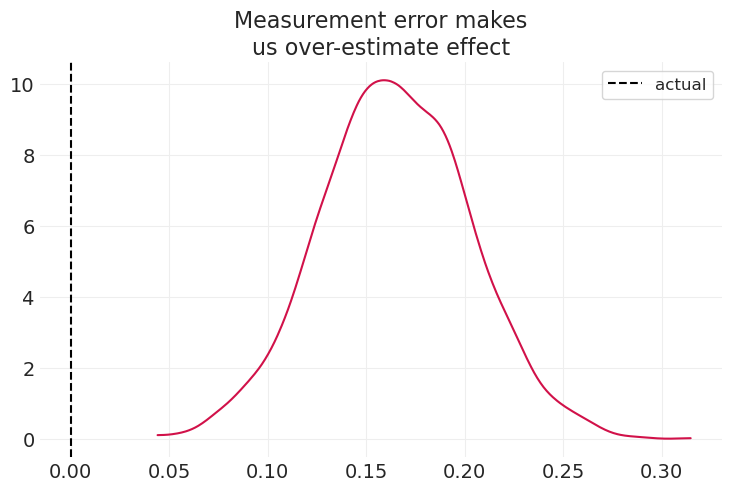
在上述情景中，测量误差可能导致我们高估实际效应

simulate_child_parent_income(beta_P=0.75, title="Measurement error makes\nus under-estimate effect")

Initializing NUTS using jitter+adapt_diag...
Multiprocess sampling (4 chains in 4 jobs)
NUTS: [sigma, beta, alpha]

Sampling 4 chains for 1_000 tune and 1_000 draw iterations (4_000 + 4_000 draws total) took 1 seconds.

	均值	标准差	hdi_3%	hdi_97%	mcse_mean	mcse_sd	ess_bulk	ess_tail	r_hat
alpha	-0.077	0.047	-0.163	0.014	0.001	0.001	5738.0	3032.0	1.0
beta	0.541	0.036	0.474	0.608	0.000	0.000	6257.0	3416.0	1.0
sigma	1.052	0.034	0.994	1.118	0.000	0.000	5247.0	2873.0	1.0

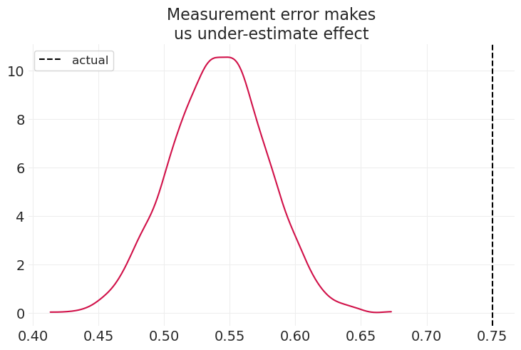
在上述情景中，测量误差可能导致我们低估实际效应

• 发生什么情况取决于具体情境的细节

• 没有通用的规则告诉你测量误差会对你的估计产生什么影响

建模测量

重温华夫饼屋离婚数据集

WAFFLE_DIVORCE = utils.load_data("WaffleDivorce")
WAFFLE_DIVORCE.head()

	地点	地点	人口	结婚年龄中位数	结婚率	结婚率标准误	离婚率	离婚率标准误	华夫饼屋数量	南方	1860 年奴隶人口	1860 年人口	1860 年奴隶比例
0	阿拉巴马州	AL	4.78	25.3	20.2	1.27	12.7	0.79	128	1	435080	964201	0.45
1	阿拉斯加州	AK	0.71	25.2	26.0	2.93	12.5	2.05	0	0	0	0	0.00
2	亚利桑那州	AZ	6.33	25.8	20.3	0.98	10.8	0.74	18	0	0	0	0.00
3	阿肯色州	AR	2.92	24.3	26.4	1.70	13.5	1.22	41	1	111115	435450	0.26
4	加利福尼亚州	CA	37.25	26.8	19.1	0.39	8.0	0.24	0	0	0	379994	0.00

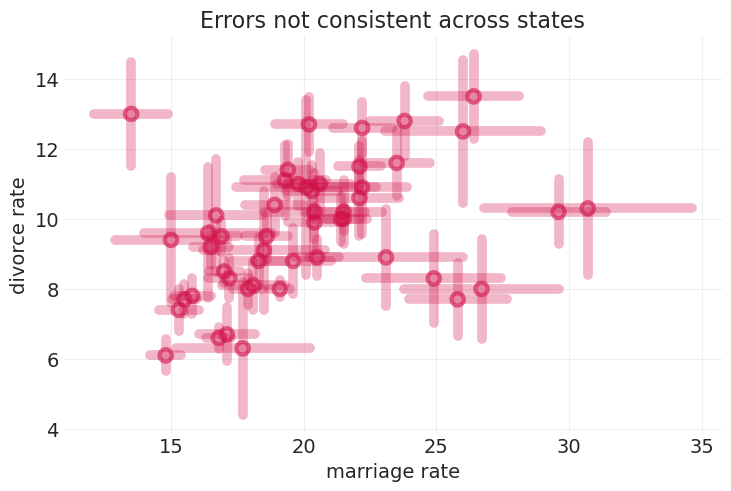
问题

• 证据不平衡

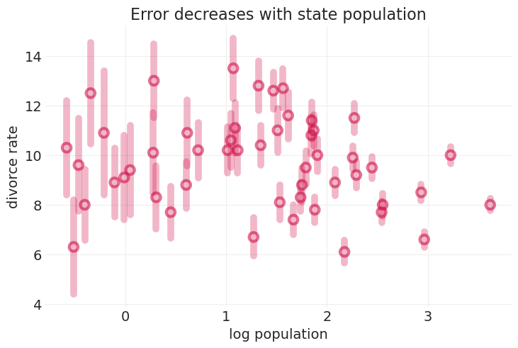
• 潜在的混淆

  • 例如，人口规模

utils.plot_scatter(WAFFLE_DIVORCE.Marriage, WAFFLE_DIVORCE.Divorce, label=None)

utils.plot_errorbar(
    xs=WAFFLE_DIVORCE.Marriage,
    ys=WAFFLE_DIVORCE.Divorce,
    error_lower=WAFFLE_DIVORCE["Divorce SE"],
    error_upper=WAFFLE_DIVORCE["Divorce SE"],
    error_width=7,
)

utils.plot_x_errorbar(
    xs=WAFFLE_DIVORCE.Marriage,
    ys=WAFFLE_DIVORCE.Divorce,
    error_lower=WAFFLE_DIVORCE["Marriage SE"],
    error_upper=WAFFLE_DIVORCE["Marriage SE"],
    error_width=7,
)

plt.xlabel("marriage rate")
plt.ylabel("divorce rate")
plt.title("Errors not consistent across states");

utils.plot_scatter(np.log(WAFFLE_DIVORCE.Population), WAFFLE_DIVORCE.Divorce, label=None)

utils.plot_errorbar(
    xs=np.log(WAFFLE_DIVORCE.Population),
    ys=WAFFLE_DIVORCE.Divorce,
    error_lower=WAFFLE_DIVORCE["Divorce SE"],
    error_upper=WAFFLE_DIVORCE["Divorce SE"],
    error_width=7,
)
plt.xlabel("log population")
plt.ylabel("divorce rate")
plt.title("Error decreases with state population");

测量的离婚模型

utils.draw_causal_graph(
    edge_list=[
        ("M", "D"),
        ("A", "M"),
        ("A", "D"),
        ("M", "M*"),
        ("D", "D*"),
        ("eD", "D*"),
        ("eM", "M*"),
        ("A", "A*"),
        ("eA", "A*"),
        ("P", "eA"),
        ("P", "eM"),
        ("P", "eD"),
        ("P", "D"),
    ],
    node_props={
        "unobserved": {"style": "dashed"},
        "A": {"style": "dashed"},
        "M": {"style": "dashed"},
        "D": {"style": "dashed"},
    },
    edge_props={
        ("P", "eA"): {"color": "blue"},
        ("P", "eM"): {"color": "blue"},
        ("P", "eD"): {"color": "blue", "label": "population confounds", "fontcolor": "blue"},
        ("P", "D"): {
            "style": "dashed",
            "label": " potential backdoor",
            "color": "red",
            "fontcolor": "red",
        },
        ("A", "A*"): {"color": "red"},
        ("P", "eA"): {"color": "purple"},
        ("eA", "A*"): {"color": "red"},
        ("A", "D"): {"color": "red"},
    },
    graph_direction="LR",
)

像图一样思考

• 像回归一样思考：我应该在模型中包含哪些预测变量？

  • 停止这样做

  • 公平地说，GLM 启用了这种方法

  • 科学世界比 GLM 大得多（例如，想想工具使用示例中的差分方程）

• 像图一样思考：我如何对原因网络进行建模？

  • 例如，完全豪华贝叶斯

让我们从更简单的开始

utils.draw_causal_graph(
    edge_list=[("M", "D"), ("A", "M"), ("A", "D"), ("M", "M*"), ("D", "D*"), ("eD", "D*")],
    node_props={
        "unobserved": {"style": "dashed"},
        "D": {"style": "dashed", "color": "red"},
        "M": {"color": "red"},
        "A": {"color": "red"},
        "eD": {"color": "blue"},
        "D*": {"color": "blue"},
    },
    edge_props={
        ("A", "M"): {"color": "red"},
        ("A", "D"): {"color": "red", "label": "Divorce Model", "fontcolor": "red"},
        ("M", "D"): {"color": "red"},
        ("eD", "D*"): {
            "color": "blue",
            "label": " Divorce Measurement\nError Model",
            "fontcolor": "blue",
        },
        ("D", "D*"): {"color": "blue"},
    },
    graph_direction="LR",
)

2 个子模型

离婚模型

\[\begin{split} \begin{align*} D_i &\sim \text{Normal}(\mu_i) \\ \mu_i &= \alpha + \beta_A A + \beta_M M \end{align*} \end{split}\]

离婚测量误差模型

\[\begin{split} \begin{align*} D^*_i &= D_i + e_D \\ e_{D,i} &\sim \text{Normal}(0, S_i) &S_i \text{ 是从样本估计的标准差} \end{align*} \end{split}\]

拟合离婚测量误差模型

• 两个同步回归

  • 一个用于 \(D\)

    • 注意：这些只是模型中的参数，它们不是观察到的 🤯

  • 一个用于 \(D*\)

DIVORCE_STD = WAFFLE_DIVORCE["Divorce"].std()
DIVORCE = utils.standardize(WAFFLE_DIVORCE["Divorce"]).values
MARRIAGE = utils.standardize(WAFFLE_DIVORCE["Marriage"]).values
AGE = utils.standardize(WAFFLE_DIVORCE["MedianAgeMarriage"]).values
DIVORCE_SE = WAFFLE_DIVORCE["Divorce SE"].values / DIVORCE_STD
STATE_ID, STATE = pd.factorize(WAFFLE_DIVORCE["Loc"])
N = len(WAFFLE_DIVORCE)

coords = {"state": STATE}
with pm.Model(coords=coords) as measured_divorce_model:
    sigma = pm.Exponential("sigma", 1)
    alpha = pm.Normal("alpha", 0, 0.2)
    beta_A = pm.Normal("beta_A", 0, 0.5)
    beta_M = pm.Normal("beta_M", 0, 0.5)

    mu = alpha + beta_A * AGE + beta_M * MARRIAGE
    D = pm.Normal("D", mu, sigma, dims="state")
    pm.Normal("D*", D, DIVORCE_SE, observed=DIVORCE)

    measured_divorce_inference = pm.sample()

Initializing NUTS using jitter+adapt_diag...
Multiprocess sampling (4 chains in 4 jobs)
NUTS: [sigma, alpha, beta_A, beta_M, D]

Sampling 4 chains for 1_000 tune and 1_000 draw iterations (4_000 + 4_000 draws total) took 1 seconds.

真实离婚率的后验分布

az.summary(measured_divorce_inference, var_names=["D"])[:10]

	均值	标准差	hdi_3%	hdi_97%	mcse_mean	mcse_sd	ess_bulk	ess_tail	r_hat
D[AL]	1.202	0.365	0.546	1.897	0.006	0.004	3821.0	2742.0	1.0
D[AK]	0.705	0.558	-0.325	1.781	0.008	0.007	4484.0	2868.0	1.0
D[AZ]	0.439	0.343	-0.197	1.076	0.005	0.004	5020.0	2553.0	1.0
D[AR]	1.443	0.478	0.587	2.366	0.007	0.005	4344.0	2760.0	1.0
D[CA]	-0.913	0.130	-1.147	-0.670	0.002	0.001	5309.0	2611.0	1.0
D[CO]	0.684	0.398	-0.054	1.416	0.006	0.005	5191.0	2965.0	1.0
D[CT]	-1.394	0.346	-2.057	-0.781	0.005	0.004	4951.0	3122.0	1.0
D[DE]	-0.329	0.504	-1.253	0.657	0.008	0.008	4483.0	3030.0	1.0
D[DC]	-1.916	0.598	-3.033	-0.761	0.010	0.007	3756.0	3303.0	1.0
D[FL]	-0.628	0.173	-0.978	-0.321	0.002	0.002	5325.0	2963.0	1.0

对离婚测量误差进行建模的效果

def plot_change_xy(x_orig, y_orig, x_new, y_new, color="C0"):
    for ii, (xo, yo, xn, yn) in enumerate(zip(x_orig, y_orig, x_new, y_new)):
        label = "change" if not ii else None
        plt.plot((xo, xn), (yo, yn), linewidth=2, alpha=0.25, color=color, label=label)


D_true = measured_divorce_inference.posterior.mean(dim=("chain", "draw"))["D"].values

# Plot raw observations
utils.plot_scatter(AGE, DIVORCE, color="k", label="observed (std)", zorder=100)

# Plot divorce posterior
utils.plot_scatter(AGE, D_true, color="C0", label="posterior mean", zorder=100)

plot_change_xy(AGE, DIVORCE, AGE, D_true)

# Add trendline
# AGE and DIVORCE are standardized, so no need for offset
trend_slope = np.linalg.lstsq(AGE[:, None], D_true)[0]
xs = np.linspace(-3, 3, 10)
ys = xs * trend_slope
utils.plot_line(xs=xs, ys=ys, linestyle="--", color="C0", label="posterior trend", linewidth=1)

plt.xlabel("marriage age (std)")
plt.ylabel("divorce rate (std)")
plt.legend();

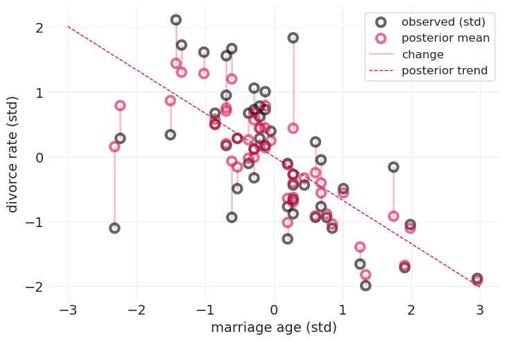
• 黑点忽略测量误差

• 红点是捕获离婚率测量误差的模型的后验均值

• 细粉色线条演示了通过建模测量误差对估计值的影响

• 对离婚率中的测量误差进行建模，会将不确定性较大（标准误差较大）的州的估计值缩小到主要趋势线（红色虚线）附近

  • 跨州的局部合并信息

• 通过绘制图形并遵循概率规则，你可以免费获得这一切

离婚率和结婚率测量误差模型

utils.draw_causal_graph(
    edge_list=[("M", "D"), ("A", "M"), ("A", "D"), ("M", "M*"), ("D", "D*"), ("eD", "D*")],
    node_props={
        "unobserved": {"style": "dashed"},
        "D": {"style": "dashed", "color": "red"},
        "M": {"color": "darkcyan"},
        "A": {"color": "darkcyan"},
        "eD": {"color": "blue"},
        "D*": {"color": "blue"},
    },
    edge_props={
        ("A", "M"): {"color": "darkcyan", "label": "Marriage Model", "fontcolor": "darkcyan"},
        ("A", "D"): {"color": "red", "label": "Divorce Model", "fontcolor": "red"},
        ("M", "D"): {"color": "red"},
        ("M", "M*"): {"label": "Marriage Measurement\nError Model"},
        ("eD", "D*"): {
            "color": "blue",
            "label": " Divorce Measurement\nError Model",
            "fontcolor": "blue",
        },
        ("D", "D*"): {"color": "blue"},
    },
    graph_direction="LR",
)

4 个子模型

离婚模型

\[\begin{split} \begin{align*} D_i &\sim \text{Normal}(\mu_{Di}, \sigma_D) \\ \mu_{Di} &= \alpha_D + \beta_{AD} A_i + \beta_{MD} M_i \end{align*} \end{split}\]

离婚测量误差模型

\[\begin{split} \begin{align*} D^*_i &= D_i + e_D \\ e_{D,i} &\sim \text{Normal}(0, S_{Di}) &S_{Di} \text{ 是从样本估计的离婚标准差} \end{align*} \end{split}\]

结婚率模型

\[\begin{split} \begin{align*} M_i &\sim \text{Normal}(\mu_{Mi}, \sigma_M) \\ \mu_{Mi} &= \alpha_M + \beta_{AM} A_i \end{align*} \end{split}\]

结婚率测量误差模型

\[\begin{split} \begin{align*} M^*_i &= M_i + e_M \\ e_{M,i} &\sim \text{Normal}(0, S_{Mi}) &S_{Mi} \text{ 是从样本估计的结婚标准差} \end{align*} \end{split}\]

MARRIAGE_STD = WAFFLE_DIVORCE["Marriage"].std()
MARRIAGE_SE = WAFFLE_DIVORCE["Marriage SE"].values / MARRIAGE_STD

coords = {"state": STATE}

with pm.Model(coords=coords) as measured_divorce_marriage_model:

    # Marriage Rate Model
    sigma_marriage = pm.Exponential("sigma_M", 1)
    alpha_marriage = pm.Normal("alpha_M", 0, 0.2)
    beta_AM = pm.Normal("beta_AM", 0, 0.5)

    # True marriage parameter
    mu_marriage = alpha_marriage + beta_AM * AGE
    M = pm.Normal("M", mu_marriage, sigma_marriage, dims="state")

    # Likelihood
    pm.Normal("M*", M, MARRIAGE_SE, observed=MARRIAGE)

    # Divorce Model
    ## Priors
    sigma_divorce = pm.Exponential("sigma_D", 1)
    alpha_divorce = pm.Normal("alpha_D", 0, 0.2)
    beta_AD = pm.Normal("beta_AD", 0, 0.5)
    beta_MD = pm.Normal("beta_MD", 0, 0.5)

    # True divorce parameter
    mu_divorce = alpha_divorce + beta_AD * AGE + beta_MD * M[STATE_ID]
    D = pm.Normal("D", mu_divorce, sigma_divorce, dims="state")

    # Likelihood
    pm.Normal("D*", D, DIVORCE_SE, observed=DIVORCE)

    measured_divorce_marriage_inference = pm.sample(target_accept=0.95)

Initializing NUTS using jitter+adapt_diag...
Multiprocess sampling (4 chains in 4 jobs)
NUTS: [sigma_M, alpha_M, beta_AM, M, sigma_D, alpha_D, beta_AD, beta_MD, D]

Sampling 4 chains for 1_000 tune and 1_000 draw iterations (4_000 + 4_000 draws total) took 3 seconds.

对离婚率和结婚率测量误差进行建模的效果

D_true = measured_divorce_marriage_inference.posterior.mean(dim=("chain", "draw"))["D"].values
M_true = measured_divorce_marriage_inference.posterior.mean(dim=("chain", "draw"))["M"].values

# Observations
utils.plot_scatter(MARRIAGE, DIVORCE, color="k", label="observed (std)", zorder=100)

# Posterior Means
utils.plot_scatter(M_true, D_true, color="C0", label="posterior mean", zorder=100)

# Change from modeling measurement error
plot_change_xy(MARRIAGE, DIVORCE, M_true, D_true)

# Add trendline
trend_slope = np.linalg.lstsq(M_true[:, None], D_true)[0]
xs = np.linspace(-3, 3, 10)
ys = xs * trend_slope
utils.plot_line(xs=xs, ys=ys, color="C0", linestyle="--", linewidth=1, label="posterior trend")

plt.xlabel("marriage rate (std)")
plt.ylabel("divorce rate (std)")
plt.legend();

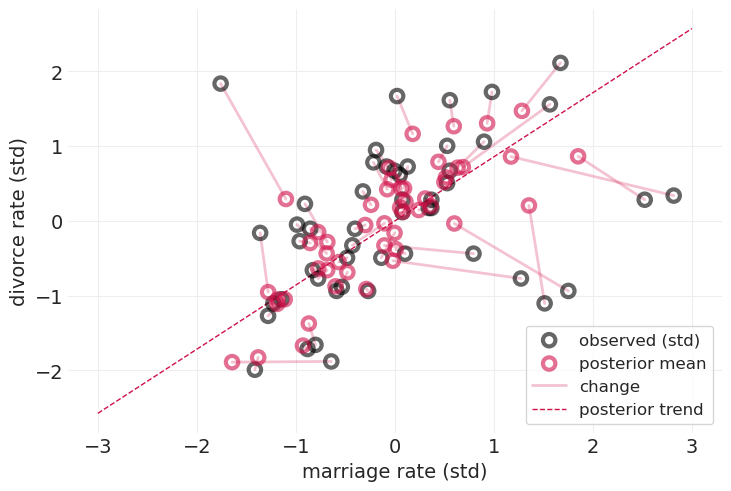
• 当对结婚率和离婚率的测量误差都进行建模时，我们得到的估计值会在多个维度上移动

• 收缩（细粉色线条）是朝向后验趋势（红色虚线）的

  • 移动方向与各自维度上的不确定性成比例

  • 移动程度与数据点的“质量”（就标准差而言）成反比

• 同样，通过写下联合分布并依靠概率公理，我们可以免费获得这一切

比较对测量误差进行建模和不进行建模的模型的因果效应

拟合不考虑测量误差的模型

with pm.Model(coords=coords) as no_measurement_error_model:

    # Divorce Model
    ## Priors
    sigma = pm.Exponential("sigma", 1)
    alpha = pm.Normal("alpha", 0, 0.2)
    beta_A = pm.Normal("beta_A", 0, 0.5)
    beta_M = pm.Normal("beta_M", 0, 0.5)

    # Likelihood
    mu = alpha + beta_A * AGE + beta_M * MARRIAGE
    pm.Normal("D", mu, sigma, observed=DIVORCE)

    no_measurement_error_model = pm.sample(target_accept=0.95)

Initializing NUTS using jitter+adapt_diag...
Multiprocess sampling (4 chains in 4 jobs)
NUTS: [sigma, alpha, beta_A, beta_M]

Sampling 4 chains for 1_000 tune and 1_000 draw iterations (4_000 + 4_000 draws total) took 1 seconds.

_, axs = plt.subplots(1, 2, figsize=(10, 5))
plt.sca(axs[0])
az.plot_dist(no_measurement_error_model.posterior["beta_A"], color="gray", label="ignoring error")
az.plot_dist(
    measured_divorce_marriage_inference.posterior["beta_AD"], color="C0", label="with error"
)
plt.axvline(0, color="k", linestyle="--", label="no effect")
plt.xlabel("$\\beta_A$")
plt.ylabel("density")
plt.legend()
axs[0].set_title("Effect of Age on Divorce Rate")

plt.sca(axs[1])
az.plot_dist(no_measurement_error_model.posterior["beta_M"], color="gray", label="ignoring error")
az.plot_dist(
    measured_divorce_marriage_inference.posterior["beta_MD"], color="C0", label="with error"
)
plt.axvline(0, color="k", linestyle="--", label="no effect")
plt.xlabel("$\\beta_M$")
plt.ylabel("density")
plt.legend()
axs[1].set_title("Effect of Marriage on Divorce Rate");

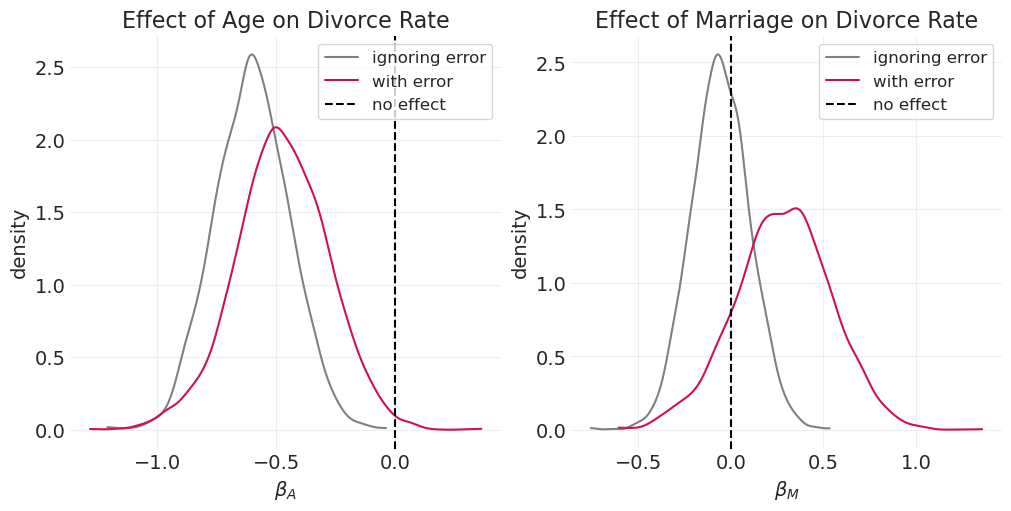
同样，对于测量误差将如何影响因果估计，没有明确的规则

• 当考虑测量误差时，年龄的估计效应会减弱（左）

• 当对测量误差进行建模时，婚姻对离婚率的估计效应会增加（右）

• 先前示例中发现的年龄和婚姻的影响可能部分是由于测量误差和/或人口混淆造成的

不可预测的误差

• 对婚姻的测量误差进行建模会增加婚姻对离婚的估计效应

  • 这不符合直觉

    • 你的直觉是魔鬼 😈

  • 通常，非线性交互的结果不符合直觉——依靠概率论

  • 可能是由于对不可靠、高不确定性的数据点进行了降权，从而改进了估计

• 误差可能会“伤害”或“帮助”，具体取决于目标

  • 唯一诚实的选择是尝试对它们进行建模

  • 尽你所能，像你希望你的同事分析他们自己的数据一样分析你的数据。

误分类

辛巴牧民文化中的亲子关系

• 不寻常的亲属关系系统（无论如何，在西方意义上）

• “开放式”婚姻

• 估计量：婚外情男人所生子女的比例 \(p\)

• 误分类：测量误差的分类版本

  • 亲子鉴定测试具有一定的假阳性率 \(f\)（FPR，例如 5%）

  • 如果婚外情亲子关系的发生率很小，则可能与 FPR 同一个数量级

    • 因此，通常不能忽略误分类误差

  • 我们如何包含误分类率？

utils.draw_causal_graph(
    edge_list=[
        ("F", "X"),
        ("F", "T"),
        ("T", "X"),
        ("M", "T"),
        ("M", "X"),
        ("X", "Xstar"),
        ("eX", "Xstar"),
    ],
    node_props={"X": {"style": "dashed"}, "unobserved": {"style": "dashed"}},
)

• 社会父亲 \(F\)

• 母亲 \(M\)

• 社会关系（二元组） \(T\)

• 实际婚外情亲子关系 \(X\)，未观察到

• 测量的婚外情亲子关系 \(X^*\)

• 误分类误差 \(e_X\)

生成模型

\[\begin{split} \begin{align*} X_i &\sim \text{Bernoulli}(p_i) \\ \text{logit}(p_i) &= \alpha + \mu_{M[i]} + \delta_{T[i]} \end{align*} \end{split}\]

测量模型

\[\begin{split} \begin{align*} P(X^*=1 | p_i) = p_i + (1 - p_i)f \\ P(X^*=0 | p_i) = (1 - p_i)(1 - f) \end{align*} \end{split}\]

其中

• 错误率 \(f\)

• 婚外情亲子关系的概率 \(p\)

以图形方式推导误分类误差模型：

不要耍小聪明，直接写出所有可能的测量结果

utils.draw_causal_graph(
    edge_list=[
        ("", "X=1"),
        ("", "X=0"),
        ("X=0", "X*=1"),
        ("X=0", "X*=0"),
    ],
    node_props={"": {"shape": "point"}},
    edge_props={
        ("", "X=1"): {"label": " p"},
        ("", "X=0"): {
            "label": " 1-p",
        },
        ("X=0", "X*=1"): {
            "label": " f",
        },
        ("X=0", "X*=0"): {"label": " 1-f"},
    },
)

\(p(X^*=1) = p + (1-p)f\)

观察到 \(X=1\) 给定 \(p\) 的概率是下面的红色路径

utils.draw_causal_graph(
    edge_list=[
        ("", "X=1"),
        ("", "X=0"),
        ("X=0", "X*=1"),
        ("X=0", "X*=0"),
    ],
    node_props={
        "": {"shape": "point"},
        "X=1": {"color": "red"},
        "X=0": {"color": "red"},
        "X*=1": {"color": "red"},
    },
    edge_props={
        ("", "X=1"): {"label": " p", "color": "red"},
        ("", "X=0"): {"label": " 1-p", "color": "red"},
        ("X=0", "X*=1"): {"label": " f", "color": "red"},
        ("X=0", "X*=0"): {"label": " 1-f"},
    },
)

\(p(X^*=0) = (1-p)(1-f)\)

观察到 \(X=0\) 给定 \(p\) 的概率是下面的红色路径

utils.draw_causal_graph(
    edge_list=[
        ("", "X=1"),
        ("", "X=0"),
        ("X=0", "X*=1"),
        ("X=0", "X*=0"),
    ],
    node_props={
        "": {"shape": "point"},
        "X=0": {"color": "red"},
        "X*=0": {"color": "red"},
    },
    edge_props={
        ("", "X=1"): {"label": " p"},
        ("", "X=0"): {"label": " 1-p", "color": "red"},
        ("X=0", "X*=0"): {"label": " 1-f", "color": "red"},
        ("X=0", "X*=1"): {"label": " f"},
    },
)

生成代理数据集

据我所知，Scelza 等人的论文中的数据集不是公开可用的，因此让我们从生成模型定义的过程模拟一个。

from itertools import product as iproduct

np.random.seed(123)

# Generate social network
N_MOTHERS = 30
N_FATHERS = 15

MOTHER_IDS = np.arange(N_MOTHERS).astype(int)
FATHER_IDS = np.arange(N_FATHERS).astype(int)

MOTHER_TRAITS = stats.norm.rvs(size=N_MOTHERS)
DYADS = np.array(list(iproduct(MOTHER_IDS, FATHER_IDS)))

N_DYADS = len(DYADS)
DYAD_ID = np.arange(N_DYADS)

RELATIONSHIPS = stats.norm.rvs(size=N_DYADS)

PATERNITY = pd.DataFrame(
    {
        "mother_id": DYADS[:, 0],
        "social_father_id": DYADS[:, 1],
        "dyad_id": DYAD_ID,
        "relationship": RELATIONSHIPS,
    }
)

# Generative model
ALPHA = 0
BETA_MOTHER_TRAIT = 1
BETA_RELATIONSHIP = 3

PATERNITY.loc[:, "mother_trait"] = PATERNITY.mother_id.apply(lambda x: MOTHER_TRAITS[x])
p_father = utils.invlogit(
    ALPHA + BETA_MOTHER_TRAIT * PATERNITY.mother_trait + BETA_RELATIONSHIP * PATERNITY.relationship
)

PATERNITY.loc[:, "p_father"] = p_father
PATERNITY.loc[:, "is_father"] = stats.bernoulli.rvs(p_father)  # unobserved actual paternity

# Measurment model
FALSE_POSITIVE_RATE = 0.05


def p_father_star(row):
    if row.is_father == 1:
        return row.p_father + (1 - row.p_father) * FALSE_POSITIVE_RATE
    return 1 - (1 - row.p_father) * (1 - FALSE_POSITIVE_RATE)


PATERNITY.loc[:, "p_father*"] = PATERNITY.apply(p_father_star, axis=1)
PATERNITY.loc[:, "is_father*"] = stats.bernoulli.rvs(p=PATERNITY["p_father*"].values)

print("Actual average paternity rate: ", PATERNITY["is_father"].mean().round(2))
print("Measured average paternity rate: ", PATERNITY["is_father*"].mean().round(2))

Actual average paternity rate:  0.48
Measured average paternity rate:  0.53

我们在上面打印出实际的和观察到的亲子关系率。 原则上，我们应该能够用我们的模型恢复这些。

PATERNITY

	mother_id	social_father_id	dyad_id	relationship	mother_trait	p_father	is_father	p_father*	is_father*
0	0	0	0	-0.255619	-1.085631	0.135581	0	0.178802	0
1	0	1	1	-2.798589	-1.085631	0.000076	0	0.050072	0
2	0	2	2	-1.771533	-1.085631	0.001658	0	0.051575	0
3	0	3	3	-0.699877	-1.085631	0.039724	0	0.087738	0
4	0	4	4	0.927462	-1.085631	0.845111	1	0.852855	0
...	...	...	...	...	...	...	...	...	...
445	29	10	445	-0.581850	-0.861755	0.068670	0	0.115236	0
446	29	11	446	-0.659560	-0.861755	0.055178	0	0.102419	1
447	29	12	447	0.750945	-0.861755	0.800764	1	0.810726	1
448	29	13	448	-2.438461	-0.861755	0.000281	0	0.050267	0
449	29	14	449	-1.307178	-0.861755	0.008299	0	0.057884	0

450 行 × 9 列

拟合具有误分类误差的模型

注释

• 我们对未知的 \(X_i\) 求平均值，因此我们没有似然性，因此模型中不需要 \(X_i \sim \text{Bernoulli}(p_i)\) 项

• 但我们仍然包含一个观测模型，其中我们使用两个基于我们的观测的同步分布

  • 如果 \(X^*=1\) 我们使用 \(p(X^*=1) = p + (1-p)f\)

  • 如果 \(X^*=0\) 我们使用 \(p(X^*=0) = (1-p)(1-f)\)

  • 为了使用这些自定义分布，我们利用 pm.Potential 函数，该函数接受每个观测分布的对数概率

    • 这类似于讲座中使用的 custom 函数

  • 我们使用下面的 vanilla 实现，一个不使用 logsumexp 等函数的实现，因为它编译得很好

MOM_ID = PATERNITY.mother_id
MOM_TRAITS = PATERNITY.mother_trait.values

with pm.Model() as paternity_measurement_model:

    beta_M = pm.TruncatedNormal("beta_M", 0, 1, lower=0.01)
    beta_T = pm.TruncatedNormal("beta_T", 0, 1, lower=0.01)

    alpha = pm.Normal("alpha", 0, 1.5)
    T = pm.Normal("T", 0, 1, shape=N_DYADS)  # Relationship strength
    M = pm.Normal("M", 0, 1, shape=N_MOTHERS)  # Mother traits

    p_father = pm.Deterministic(
        "p_father", pm.math.invlogit(alpha + M[MOM_ID] * beta_M + T[DYAD_ID] * beta_T)
    )

    custom_log_p_x1 = pm.math.log(p_father + (1 - p_father) * FALSE_POSITIVE_RATE)
    pm.Potential("X*=1", custom_log_p_x1)

    custom_log_p_x0 = pm.math.log((1 - p_father) * (1 - FALSE_POSITIVE_RATE))
    pm.Potential("X*=0", custom_log_p_x0)

    paternity_measurement_inference = pm.sample(target_accept=0.95)

Initializing NUTS using jitter+adapt_diag...
Multiprocess sampling (4 chains in 4 jobs)
NUTS: [beta_M, beta_T, alpha, T, M]

Sampling 4 chains for 1_000 tune and 1_000 draw iterations (4_000 + 4_000 draws total) took 4 seconds.
The rhat statistic is larger than 1.01 for some parameters. This indicates problems during sampling. See https://arxiv.org/abs/1903.08008 for details

拟合不考虑误分类的类似模型

IS_FATHER_STAR = PATERNITY["is_father*"].values
with pm.Model() as paternity_model:

    alpha = pm.Normal("alpha", 0, 1.5)
    beta_M = pm.TruncatedNormal("beta_M", 0, 1, lower=0.01)
    beta_T = pm.TruncatedNormal("beta_T", 0, 1, lower=0.01)

    T = pm.Normal("T", 0, 1, shape=N_DYADS)  # Relationship strength
    M = pm.Normal("M", 0, 1, shape=N_MOTHERS)  # Mother traits

    p_father = pm.Deterministic(
        "p_father", pm.math.invlogit(alpha + M[MOM_ID] * beta_M + T[DYAD_ID] * beta_T)
    )
    pm.Bernoulli("is_father", p_father, observed=IS_FATHER_STAR)

    paternity_inference = pm.sample(target_accept=0.95)

Initializing NUTS using jitter+adapt_diag...
Multiprocess sampling (4 chains in 4 jobs)
NUTS: [alpha, beta_M, beta_T, T, M]

Sampling 4 chains for 1_000 tune and 1_000 draw iterations (4_000 + 4_000 draws total) took 7 seconds.
There were 6 divergences after tuning. Increase `target_accept` or reparameterize.
The rhat statistic is larger than 1.01 for some parameters. This indicates problems during sampling. See https://arxiv.org/abs/1903.08008 for details
The effective sample size per chain is smaller than 100 for some parameters.  A higher number is needed for reliable rhat and ess computation. See https://arxiv.org/abs/1903.08008 for details

plt.subplots(figsize=(10, 4))
az.plot_dist(paternity_inference.posterior["p_father"], color="k")
p_father_mean = paternity_inference.posterior["p_father"].mean()
plt.axvline(
    p_father_mean,
    color="k",
    linestyle="--",
    label=f"Without Measurement Error: {p_father_mean:1.2f}",
)

az.plot_dist(paternity_measurement_inference.posterior["p_father"])
p_father_mean = paternity_measurement_inference.posterior["p_father"].mean()
plt.axvline(p_father_mean, linestyle="--", label=f"With Measurement Error: {p_father_mean:1.2f}")
plt.xlim([0, 1])
plt.legend()

plt.legend()

print("Actual average paternity rate: ", PATERNITY["is_father"].mean().round(2))
print("Measured average paternity rate: ", PATERNITY["is_father*"].mean().round(2))

Actual average paternity rate:  0.48
Measured average paternity rate:  0.53

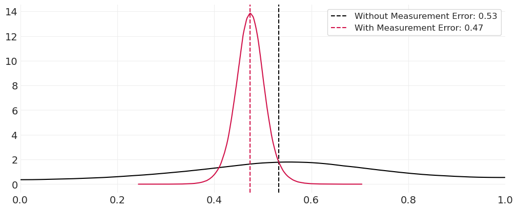
• 包括测量误差，我们能够准确地恢复实际平均亲子关系率。

• 如果不将测量误差包含在模型中，我们会恢复在存在误分类误差的情况下观察到的亲子关系率。

• 至少对于这个模拟数据集，与模型中不建模误分类误差相比，包括测量误差为我们提供了更严格的估计亲子关系率的后验分布。

测量与误分类的范围

有许多与建模测量误差和误分类相关的问题和解决方案

• 项目反应理论 (IRT)

  • 例如，之前的 NJ 葡萄酒评判示例

• 因子分析

• 障碍模型

  • 测量需要跨越阈值才能被识别

• 占用模型

  • 考虑现象的存在而无需检测

  • 在应用生态学中很重要：仅仅因为没有检测到某个物种，并不意味着它不存在

奖励：浮点怪物

• 在对数刻度上工作可以避免（或者说，最大限度地减少）与浮点运算溢出（四舍五入为 1）或下溢（四舍五入为零）相关的问题

• “古代武器”：用于对数刻度工作的特殊函数

  • pm.logsumexp：有效地计算输入元素的指数和的对数。

  • pm.math.log1mexp：计算 \(\log(1 - \exp(-x))\)

  • pm.log(1 - p)

对数是有意义的

\[\begin{split} \begin{align*} P(X^*=0) &= (1-p)(1-f) \\ \log P(X^*=0) & = \log (1-p) + \log (1-f) &\text{放在对数刻度上（HMC 使用）} \end{align*} \end{split}\]

细节决定成败

某些项可能在数值上变得不稳定

• 例如，如果 \(p \approx 0, \log(1-p) \approx \log(1) = 0\)

• 例如，如果 \(p \approx 1, \log(1-p) \approx \log(0) = -\infty\)

for p in [1e-2, 1e-10, 1e-90]:
    print("p:", p, ", log(1-p):", np.log(1 - p))

p: 0.01 , log(1-p): -0.01005033585350145
p: 1e-10 , log(1-p): -1.000000082790371e-10
p: 1e-90 , log(1-p): 0.0

def log1m(x):
    return np.log1p(-x)


for p in [1e-2, 1e-10, 1e-90]:
    print("p:", p, ", log1p(1-p):", log1m(p))

p: 0.01 , log1p(1-p): -0.010050335853501442
p: 1e-10 , log1p(1-p): -1.00000000005e-10
p: 1e-90 , log1p(1-p): -1e-90

log1p 和小 \(p\) 的泰勒级数近似

• 当 \(p>e{-4}\) 时，只需计算 \(\log(1 + p)\)

• 当 \(p<e{-4}\) 时，使用泰勒展开式：\(\log(1 + p) = p - \frac{p^2}{2} + \frac{p^3}{3} - ...\)

def my_log1p(x):
    if x > 1e-4:
        return np.log(1 + x)
    else:
        # second order Taylor expansion
        return x - x**2 / 2


# Compare results to numpy log1p
for p in [1e-3, 1e-10, 1e-90]:
    print("p:", p, ", numpy.log1p:", np.log1p(p), ", my_log1p", my_log1p(p))

p: 0.001 , numpy.log1p: 0.0009995003330835331 , my_log1p 0.0009995003330834232
p: 1e-10 , numpy.log1p: 9.999999999500001e-11 , my_log1p 9.999999999500001e-11
p: 1e-90 , numpy.log1p: 1e-90 , my_log1p 1e-90

logsumexp

• 当需要计算多个项的对数之和时使用。

• 想要对数是因为它在数值上会很稳定

• 但对数不适用于和，仅适用于积，例如

\[\begin{split} \begin{align*} P(X^*=1) &= p + (1-p)f \\ \log P(X^*=1) &= \log [p + (1-p)f] \\ \log P(X^*=1) &= \text{pm.math.logsumexp}([\text{pm.math.log}(p), \text{pm.math.log}(1-p) + \text{pm.math.log}(f))]) \\ \log P(X^*=1) &= \text{pm.math.logsumexp}([\text{pm.math.log}(p), \text{log1m}(p)) + \text{pm.math.log}(f))]) \end{align*} \end{split}\]

带有对数缩放技巧的先前亲子关系测量模型

p_father = 0.5
# pm.math.logsumexp((pm.math.log(p_father), log1m(p_father) + )).eval()
pm.math.log(FALSE_POSITIVE_RATE).astype("float32").eval()

array(-2.9957323, dtype=float32)

MOM_ID = PATERNITY.mother_id

with pm.Model() as paternity_measurement_lse_model:

    beta_M = pm.TruncatedNormal("beta_M", 0, 1, lower=0.01)
    beta_T = pm.TruncatedNormal("beta_T", 0, 1, lower=0.01)

    alpha = pm.Normal("alpha", 0, 1.5)
    T = pm.Normal("T", 0, 1, shape=N_DYADS)  # Relationship strength
    M = pm.Normal("M", 0, 1, shape=N_MOTHERS)  # Mother traits

    p = pm.Deterministic("p", pm.math.invlogit(alpha + M[MOM_ID] * beta_M + T[DYAD_ID] * beta_T))
    f = FALSE_POSITIVE_RATE

    # # For reference: the original custom logp with vanilla parameterization
    # custom_log_p_x1 = pm.math.log(p + (1 - p) * f)
    # custom_log_p_x0 = pm.math.log((1 - p) * (1 - f))

    # Custom logp using log-space reparameterization
    custom_log_p_x1 = pm.math.logsumexp(
        [pm.math.log(p), pt.math.log1p(-p) + pm.math.log(f)], axis=0
    )  # this line is problematic
    # First compute (1-p)*f in log space, then combine with p
    custom_log_p_x0 = pt.math.log1p(-p) + pt.math.log1p(-f)

    pm.Potential("X*=1", custom_log_p_x1)
    pm.Potential("X*=0", custom_log_p_x0)

    paternity_measurement_lse_inference = pm.sample(target_accept=0.95)

Initializing NUTS using jitter+adapt_diag...
Multiprocess sampling (4 chains in 4 jobs)
NUTS: [beta_M, beta_T, alpha, T, M]

Sampling 4 chains for 1_000 tune and 1_000 draw iterations (4_000 + 4_000 draws total) took 7 seconds.

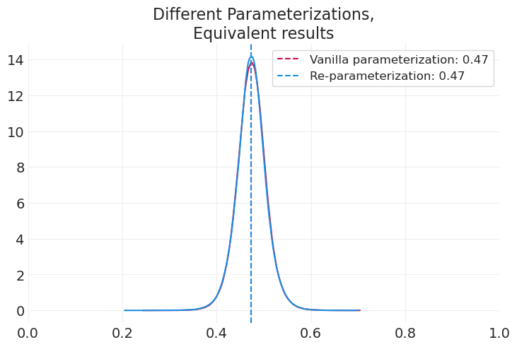
# Original vanilla parameterization
az.plot_dist(paternity_measurement_inference.posterior["p_father"])
p_father_mean = paternity_measurement_inference.posterior["p_father"].mean()
plt.axvline(p_father_mean, linestyle="--", label=f"Vanilla parameterization: {p_father_mean:1.2f}")

# Re-parameterization
az.plot_dist(paternity_measurement_lse_inference.posterior["p"], color="C1")
p_father_mean = paternity_measurement_lse_inference.posterior["p"].mean()
plt.axvline(
    p_father_mean, linestyle="--", color="C1", label=f"Re-parameterization: {p_father_mean:1.2f}"
)
plt.xlim([0, 1])

plt.legend()
plt.title("Different Parameterizations,\nEquivalent results");

作者

• 移植到 PyMC：Dustin Stansbury (2024)

• 基于 Richard McElreath 的 Statistical Rethinking (2023) 讲座

%load_ext watermark
%watermark -n -u -v -iv -w -p pytensor,aeppl,xarray

Last updated: Thu Feb 20 2025

Python implementation: CPython
Python version       : 3.12.9
IPython version      : 8.32.0

pytensor: 2.27.1
aeppl   : not installed
xarray  : 2025.1.2

arviz      : 0.19.0
xarray     : 2025.1.2
scipy      : 1.15.2
pytensor   : 2.27.1
numpy      : 1.26.4
pymc       : 5.20.1
statsmodels: 0.14.4
matplotlib : 3.10.0
pandas     : 2.2.3

Watermark: 2.5.0

许可证声明

此示例库中的所有笔记本均根据 MIT 许可证 提供，该许可证允许修改和再分发用于任何用途，前提是保留版权和许可证声明。

引用 PyMC 示例

要引用此笔记本，请使用 Zenodo 为 pymc-examples 存储库提供的 DOI。

重要提示

许多笔记本改编自其他来源：博客、书籍…… 在这种情况下，您也应该引用原始来源。

另请记住引用您的代码使用的相关库。

这是一个 bibtex 中的引用模板

@incollection{citekey,
  author    = "<notebook authors, see above>",
  title     = "<notebook title>",
  editor    = "PyMC Team",
  booktitle = "PyMC examples",
  doi       = "10.5281/zenodo.5654871"
}

一旦渲染，它可能看起来像