缺失数据#

此 notebook 是 PyMC 端口的一部分，该端口移植了 Richard McElreath 的Statistical Rethinking 2023 系列讲座。

# Ignore warnings
import warnings

import arviz as az
import numpy as np
import pandas as pd
import pymc as pm
import statsmodels.formula.api as smf
import utils as utils
import xarray as xr

from matplotlib import pyplot as plt
from matplotlib import style
from scipy import stats as stats

warnings.filterwarnings("ignore")

# Set matplotlib style
STYLE = "statistical-rethinking-2023.mplstyle"
style.use(STYLE)

缺失数据，已找到#

观测数据是一种特殊情况
- 我们欺骗自己相信没有误差
- 无/小误差是罕见的

大多数数据都缺失

但仍然有关于缺失数据的信息。在生成模型中，没有数据是完全缺失的

约束 - 例如，身高永远不会为负，并且是有界的
与其他变量的关系 - 例如，天气影响我们的行为，我们的行为不会影响天气

处理缺失数据是一个工作流程#

如何处理缺失数据？#

完整案例分析：删除缺失值的案例
- 有时是正确的做法
- 取决于上下文和因果假设
插补：用基于现有值的合理值填充缺失值
- 通常对于准确估计是必要且有益的

狗吃了我的作业：查看不同的缺失数据情景#

utils.draw_causal_graph(
    edge_list=[("S", "H"), ("H", "H*"), ("D", "H*")],
    node_props={
        "S": {"color": "red"},
        "H*": {"color": "red"},
        "H": {"style": "dashed"},
        "unobserved": {"style": "dashed"},
    },
    edge_props={
        ("S", "H"): {"color": "red"},
        ("H", "H*"): {"color": "red"},
    },
    graph_direction="LR",
)

../_images/532bd0c84288d1b25783737ab096b208daa2532a061c961af2c360e0ac29521a.svg

学生能力/知识状态 \(S\)
学生将在家庭作业中获得分数 \(H\)
我们只能观察到老师看到的家庭作业 \(H^*\)
- 我们无法观察到真实的分数，因为家庭作业可能无法到达老师手中
- 例如，家里的狗 \(D\) 随机吃掉家庭作业（缺失机制）

狗通常是良性的#

# Helper functions
def plot_regression_line(x, y, color, label, **plot_kwargs):
    valid_idx = ~np.isnan(y)

    X = np.vstack((np.ones_like(x[valid_idx]), x[valid_idx])).T
    intercept, slope = np.linalg.lstsq(X, y[valid_idx])[0]

    xs = np.linspace(x.min(), x.max(), 10)
    ys = xs * slope + intercept
    utils.plot_line(xs, ys, color=color, label=label, **plot_kwargs)


def plot_dog_homework(S, H, Hstar, title=None):

    utils.plot_scatter(S, H, color="k", alpha=1, label="total", s=10)
    plot_regression_line(S, H, label="total trend", color="k", alpha=0.5)

    utils.plot_scatter(S, Hstar, color="C0", alpha=0.8, label="incomplete")
    plot_regression_line(S, Hstar, label="incomplete trend", color="C0", alpha=0.5)

    plt.xlabel("S")
    plt.ylabel("H")
    plt.title(title)
    plt.legend();

模拟随机吃作业#

np.random.seed(123)
n_homework = 100
# Student knowledge
S = stats.norm.rvs(size=n_homework)

# Homework score
mu_score = S * 0.5
H = stats.norm.rvs(mu_score)

# Dog eats 50% of of homework _at random_
D = stats.bernoulli(0.5).rvs(size=n_homework)
Hstar = H.copy()
Hstar[D == 1] = np.nan

plot_dog_homework(
    S, H, Hstar, title="Random missing data\ncauses loss of precision; little/no bias"
)

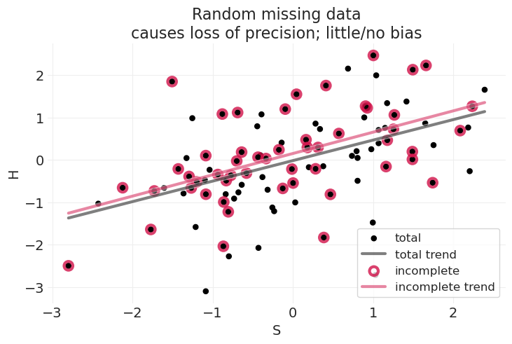
../_images/f38c8113377d38790542b2d1414fa30bf8ac0f2656ba1be613f54ab0ee8e0250.png

当随机丢失结果时，我们获得类似的线性拟合，具有相似的斜率，并且没有或几乎没有偏差。
因此，删除完整案例是可以的，但会降低效率

狗根据家庭作业的原因（学生能力）吃家庭作业#

现在学生的能力影响了狗的行为（例如，学生学习太多而没有喂狗，狗饿了）

utils.draw_causal_graph(
    edge_list=[("S", "H"), ("H", "H*"), ("D", "H*"), ("S", "D")],
    node_props={
        "S": {"color": "blue"},
        "H*": {"color": "red"},
        "H": {"style": "dashed"},
        "unobserved": {"style": "dashed"},
    },
    edge_props={
        ("S", "H"): {"color": "red"},
        ("H", "H*"): {"color": "red"},
        ("S", "D"): {"color": "blue", "label": "possible biasing path", "fontcolor": "blue"},
        ("D", "H*"): {"color": "blue"},
    },
    graph_direction="LR",
)

../_images/687bbb0713b1011c8e314be2615fca9bf4e1680af0dd7c8f45a96241358fb2c5.svg

模拟治疗效果线性影响结果的数据#

np.random.seed(12)
n_homework = 100
# Student knowledge
S = stats.norm.rvs(size=n_homework)

# Linear association between student ability and homework score
mu_score = S * 0.5
H = stats.norm.rvs(mu_score)

# Dog eats based on the student's ability
p_dog_eats_homework = np.where(S > 0, 0.9, 0)
D = stats.bernoulli.rvs(p=p_dog_eats_homework)
Hstar = H.copy()
Hstar[D == 1] = np.nan

plot_dog_homework(
    S,
    H,
    Hstar,
    title="Missing data conditioned on common cause\nmay work for linear relationships (rare) ",
)

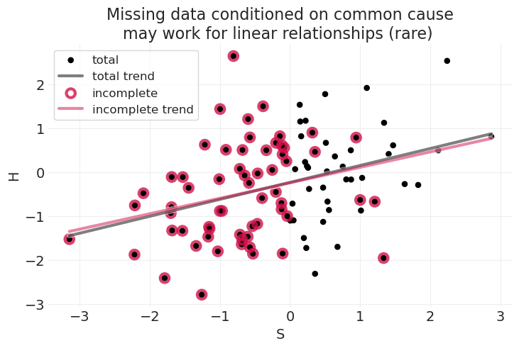
../_images/9bd849c4283f5576b86592de22d4f1a881e3858614ee50fb8288edff4edddc5e.png

当学生能力 \(S\) 和家庭作业分数 \(H\) 之间的关联是线性关系时，我们仍然可以从总样本和不完整样本中获得相当相似的线性拟合，只是在 \(S\) 维度的上限上损失了一些精度，在本模拟中

模拟治疗效果非线性影响结果的数据#

np.random.seed(1)
n_homework = 100
# Student knowledge
S = stats.norm.rvs(size=n_homework)

# Nonlinear association between student ability and homework score
mu_score = 1 - np.exp(-0.7 * S)
H = stats.norm.rvs(mu_score)

# Dog eats all the homework of above-average students
p_dog_eats_homework = np.where(S > 0, 1, 0)
D = stats.bernoulli.rvs(p=p_dog_eats_homework)
Hstar = H.copy()
Hstar[D == 1] = np.nan

plot_dog_homework(
    S,
    H,
    Hstar,
    title="Missing data based on common cause\nvery bady for non-linear relationships (common)",
)

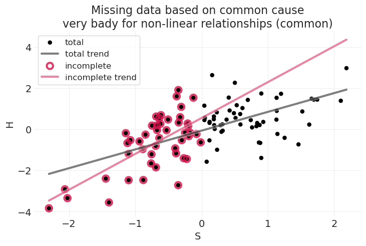
../_images/826a97d3ed02a25930a34baa411ea42c33dda1aa9c95e10c11f84a7ff92e5bfa.png

当学生能力 \(S\) 和家庭作业分数 \(H\) 之间的关联是非线性关系时，我们现在从总样本和不完整样本中获得非常不同的线性拟合
- 关于非线性：这就是为什么我们使用具有科学动机函数的生成模型：函数很重要
因此，需要正确地以原因为条件

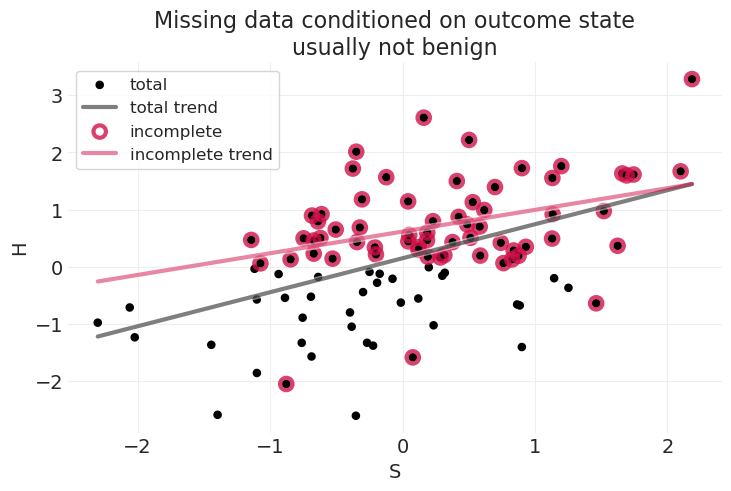
狗根据家庭作业状态本身来吃家庭作业#

utils.draw_causal_graph(
    edge_list=[("S", "H"), ("H", "H*"), ("D", "H*"), ("H", "D")],
    node_props={
        "H*": {"color": "red"},
        "H": {"style": "dashed"},
        "unobserved": {"style": "dashed"},
    },
    edge_props={
        ("S", "H"): {"color": "red"},
        ("H", "H*"): {"color": "red"},
        ("H", "D"): {"color": "blue", "label": "biasing path", "fontcolor": "blue"},
        ("D", "H*"): {"color": "blue"},
    },
    graph_direction="LR",
)

../_images/5c91b8d3538cc5781ace06a67acaa12e32a45fc7812062c51171a8f024b4fd5b.svg

模拟一些线性数据#

np.random.seed(1)
n_homework = 100
# Student knowledge
S = stats.norm.rvs(size=n_homework)

# Linear association between ability and score
mu_score = S * 0.5
H = stats.norm.rvs(mu_score)

# Dog eats 90% of homework that is below average
p_dog_eats_homework = np.where(H < 0, 0.9, 0)
D = stats.bernoulli.rvs(p=p_dog_eats_homework)
Hstar = H.copy()
Hstar[D == 1] = np.nan

plot_dog_homework(
    S, H, Hstar, title="Missing data conditioned on outcome state\nusually not benign"
)

../_images/a9a9f43d8c4ead4b6e4a02ca71e8b370ad5e3d27ba866f9df8d746c2c2dd6ee3.png

np.random.seed(1)
n_homework = 100
# Student knowledge
S = stats.norm.rvs(size=n_homework)

# Nonlinear association between student ability and homework score
mu_score = 1 - np.exp(-0.9 * S)
H = stats.norm.rvs(mu_score)

# Dog eats 90% of homework that is below average
p_dog_eats_homework = np.where(H < 0, 0.9, 0)
D = stats.bernoulli.rvs(p=p_dog_eats_homework)
Hstar = H.copy()
Hstar[D == 1] = np.nan

plot_dog_homework(
    S,
    H,
    Hstar,
    title="Missing data conditioned on outcome state\nsimilar for nonlinear relationships",
)

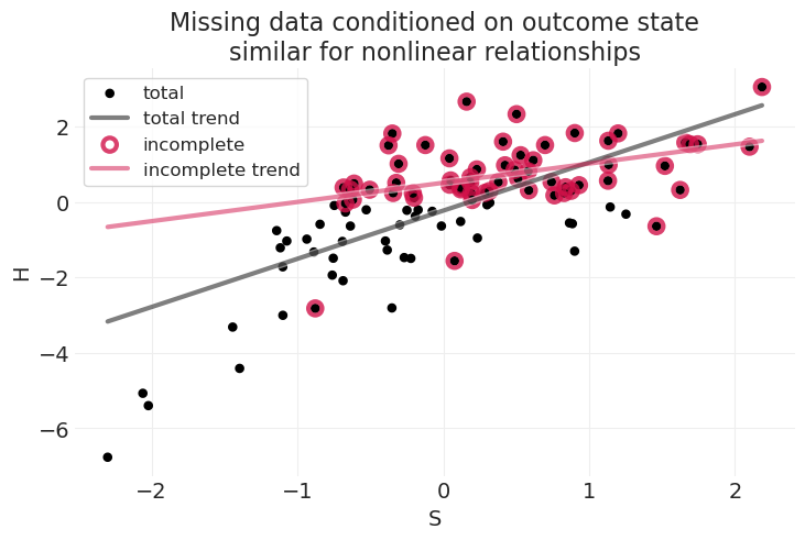
../_images/a42a1538d1b1c7f5728e3bc6c8f3ac147404b14ee762b7597af27b07bb87e35f.png

在不知道状态与数据丢失之间的因果关系，以及 \(S\) 如何与 \(H\) 相关联的函数形式的情况下，很难解释这种情况

典型案例#

数据丢失是随机的且独立于原因
- “狗随机吃家庭作业”
- 删除完整案例是可以的，但会降低效率
数据丢失以原因为条件
- “狗根据学生的学习习惯吃家庭作业”
- 需要正确地以原因为条件
数据丢失以结果为条件
- “狗根据家庭作业的分数吃家庭作业”
- 除非我们可以对状态如何影响数据丢失的因果过程（即本模拟中狗的行为）进行建模，否则这通常是无望的
  - 例如，生存分析和删失数据

贝叶斯插补#

适用于典型案例 1）、2）和 3）的子集（例如，生存分析）
拥有所有变量（观测数据和参数）的联合（贝叶斯）模型，为推断缺失值的合理范围提供了方法

插补或边缘化#

插补：计算缺失值的后验概率分布
- 通常涉及部分合并
- 我们已经在孟加拉国数据集的缺失地区中在某种程度上做到了这一点
边缘化未知数：使用其他变量的后验分布，对缺失值的分布求平均值
- 无需计算缺失值的后验分布

何时插补？何时边缘化？#

有时插补是不必要的 – 例如，离散变量
- 边缘化在这里有效
有时插补更容易
- 例如，当数据丢失过程像生存分析中的删失那样被很好地理解时
- 对于更奇特的模型，边缘化可能很困难

重新审视系统发育回归#

PRIMATES301 = utils.load_data("Primates301")
PRIMATES301.head()

	名称	属	物种	亚种	spp_id	genus_id	研究投入	大脑	身体	群体大小	妊娠期	断奶期	寿命	性成熟期	母体投入
0	Allenopithecus_nigroviridis	Allenopithecus	nigroviridis	NaN	1	1	6.0	58.02	4655.00	40.0	NaN	106.15	276.0	NaN	NaN
1	Allocebus_trichotis	Allocebus	trichotis	NaN	2	2	6.0	NaN	78.09	1.0	NaN	NaN	NaN	NaN	NaN
2	Alouatta_belzebul	Alouatta	belzebul	NaN	3	3	15.0	52.84	6395.00	7.4	NaN	NaN	NaN	NaN	NaN
3	Alouatta_caraya	Alouatta	caraya	NaN	4	3	45.0	52.63	5383.00	8.9	185.92	323.16	243.6	1276.72	509.08
4	Alouatta_guariba	Alouatta	guariba	NaN	5	3	37.0	51.70	5175.00	7.4	NaN	NaN	NaN	NaN	NaN

301 种灵长类动物概况
生命史特征
- 体重 \(M\)
- 大脑大小 \(B\)
- 社会群体大小 \(G\)
问题
- 大量缺失数据
  - 完整案例分析仅包括 151 个观测值
- 测量误差
- 未观测到的混淆

插补灵长类动物#

核心思想：缺失值具有概率分布
- 为每个部分观测到的变量表达一个因果模型
- 用参数替换每个缺失值，并让模型像往常一样进行
  - 参数和数据的二元性
    - 在贝叶斯方法中，参数和数据之间没有区别：缺失值只是一个参数，观测值是数据
- 例如，一个可用的变量可以告知我们与观测值相关的缺失变量的合理值
概念上很奇怪，技术上很笨拙

重新审视之前的因果模型#

utils.draw_causal_graph(
    edge_list=[("G", "B"), ("M", "B"), ("M", "G"), ("u", "M"), ("u", "G"), ("u", "B"), ("H", "u")],
    graph_direction="LR",
)

../_images/a8432fe88a0d0ba9c7814260455d4979fca51463507820ee9723e6208e35a4e7.svg

其中 \(M,G,B\) 如上定义
共享历史 \(H\)，这导致
基于历史的混淆因素 \(u\)，我们尝试用系统发育来捕获它

现在让我们包括缺失值可能如何发生#

utils.draw_causal_graph(
    edge_list=[
        ("G", "B"),
        ("M", "B"),
        ("M", "G"),
        ("u", "M"),
        ("u", "G"),
        ("u", "B"),
        ("H", "u"),
        ("G", "G*"),
        ("mG", "G*"),
    ],
    graph_direction="LR",
)

../_images/4d8070121224953171afd7209f121e628701a5990ef08ce64ceb0c65fa50b507.svg

我们观察到群体大小 \(G^*\)，对于某些观测值/物种，它具有缺失值
什么影响了缺失的原因 \(m_G\)？
- 通常的假设是它是完全随机的，但这极不可能
- 缺失可能以多种方式发生。

关于是什么导致数据缺失的一些假设…#

utils.draw_causal_graph(
    edge_list=[
        ("G", "B"),
        ("M", "B"),
        ("M", "G"),
        ("u", "M"),
        ("u", "G"),
        ("u", "B"),
        ("H", "u"),
        ("G", "G*"),
        ("mG", "G*"),
        ("M", "mG"),
        ("u", "mG"),
        ("G", "mG"),
    ],
    edge_props={
        ("u", "mG"): {"color": "blue", "fontcolor": "blue", "label": "anthro-narcisism"},
        ("M", "mG"): {"color": "darkcyan", "fontcolor": "darkcyan", "label": "larger species"},
        ("G", "mG"): {"color": "red", "fontcolor": "red", "label": "solitary species"},
    },
    graph_direction="LR",
)

../_images/b4325eb046ea82d5557eaab0d6d7249d83b5fd8274f53cc9fa8af6205d2469b6.svg

所有彩色箭头以及假设/推测都可能在起作用
- 人类中心主义：人类更可能研究与他们相似的灵长类动物
- 体型较大的物种，体重较大，更容易计数：例如，某些物种可能生活在树上，更难观察
- 某些物种几乎没有或没有社会群体；这些独居物种很难观察和收集数据
无论假设如何，目标是使用因果模型来推断每个缺失值的概率分布
每个缺失值的不确定性将贯穿整个模型
- 再说一次，无需聪明
- 信任概率公理

同时为多个变量建模缺失数据#

\(M, G, B\) 都具有缺失值 \(M^, G^, B^*\)#

utils.draw_causal_graph(
    edge_list=[
        ("M", "G"),
        ("M", "B"),
        ("G", "B"),
        ("M", "M*"),
        ("G", "G*"),
        ("B", "B*"),
        ("mM", "M*"),
        ("mB", "B*"),
        ("mG", "G*"),
        ("H", "u"),
        ("u", "G"),
        ("u", "M"),
        ("u", "B"),
    ],
    node_props={
        "G": {"style": "dashed"},
        "M": {"style": "dashed"},
        "B": {"style": "dashed"},
        "unobserved": {"style": "dashed"},
    },
    graph_direction="LR",
)

../_images/1952cd1865845d2cc0a0ff373a0df817bb19d717d1db8eb86d5b9a25d17cd8ba.svg

处理大脑大小 \(B\) 中的缺失值#

事实证明，我们在最初的系统发育回归示例中已经使用高斯过程处理了这个问题。通过利用高斯过程提供的局部合并，我们使用与缺失值的物种相似的物种的信息来填充缺失的大脑大小 \(B\) 值，但确实具有 \(B\) 的值。

用于在第 16 讲 - 高斯过程的“系统发育回归”部分建模大脑大小的等效因果子图

大脑大小 \(B\) 模型#

假设缺失完全是随机的

utils.draw_causal_graph(
    edge_list=[("G", "B"), ("M", "B"), ("u, D", "B"), ("H", "u, D")], graph_direction="LR"
)

../_images/8380dcc2e52d18f81e34fcc47d2a86c9e43fb87c6798f5b0f68a4212a17b01d8.svg

\[\begin{split} \begin{align} \textbf{B} &\sim \text{MVNormal}(\mu_B, \textbf{K}_B) \\ \mu_{B,i} &= \alpha_B + \beta_{GB} G_i + \beta_{MB} M_i \\ \mathbf{K}_B &= \eta_B^2 \exp(-\rho_B D_{jk})\\ \alpha_B &\sim \text{Normal}(0, 1) \\ \beta_{GB, MB} &\sim \text{Normal}(0, 1) \\ \eta_B^2 &\sim \text{HalfNormal}(1, 0.25)\\ \rho_B &\sim \text{HalfNormal}(3, 0.25) \end{align} \end{split}\]

我们可以使用类似的方法，同时为其他可能具有缺失值的变量 \(G,M\) 公式化并行模型，类似于完全豪华贝叶斯方法。

群体大小 \(G\) 模型#

utils.draw_causal_graph(edge_list=[("M", "G"), ("u, D", "G"), ("H", "u, D")], graph_direction="LR")

../_images/cbc11b16a519f93131c5506268ee04b5dc7a2f6eba35df44cffa3a684c5ae9d2.svg

\[\begin{split} \begin{align} \textbf{G} &\sim \text{MVNormal}(\mu_G, \textbf{K}_G) \\ \mu_{G,i} &= \alpha_G + \beta_{MG} M_i \\ \mathbf{K}_G &= \eta_G^2 \exp(-\rho_G D_{jk})\\ \alpha_G &\sim \text{Normal}(0, 1) \\ \beta_{MG} &\sim \text{Normal}(0, 1) \\ \eta_G^2 &\sim \text{HalfNormal}(1, 0.25)\\ \rho_G &\sim \text{HalfNormal}(3, 0.25) \end{align} \end{split}\]

体重 \(M\) 模型#

utils.draw_causal_graph(edge_list=[("u, D", "M"), ("H", "u, D")], graph_direction="LR")

../_images/41c538db3aa647e0a24b0d9ba28e5ace56651185fe32c6ab17c651cbf336b173.svg

\[\begin{split} \begin{align} \textbf{M} &\sim \text{MVNormal}(\mathbf{0}, \textbf{K}_M) \\ \mathbf{K}_M &= \eta_M^2 \exp(-\rho_M D_{jk})\\ \eta_M^2 &\sim \text{HalfNormal}(1, 0.25)\\ \rho_M &\sim \text{HalfNormal}(3, 0.25) \end{align} \end{split}\]

绘制缺失的猫头鹰 🦉#

构建包含三个同步高斯过程的模型有很多工作部分。最好以小步骤建立模型复杂性。

忽略缺少 \(B\) 值的案例（目前）
- \(B\) 是结果，因此任何插补都只是预测
插补 \(G,M\)，忽略每个模型的模型
- 错误的模型，正确的流程
- 使我们能够看到向模型添加复杂性的后果
使用 \(G\) 特定的子模型插补 \(G\)
使用每个子模型插补 \(B,G,M\)

1. 忽略缺少 \(B\) 值的案例#

筛选掉缺少大脑体积测量的观测值#

PRIMATES = PRIMATES301[PRIMATES301.brain.notna()]
PRIMATES

	名称	属	物种	亚种	spp_id	genus_id	社会学习	研究投入	大脑	身体	群体大小	妊娠期	断奶期	寿命	性成熟期	母体投入
0	Allenopithecus_nigroviridis	Allenopithecus	nigroviridis	NaN	1	1	0.0	6.0	58.02	4655.0	40.00	NaN	106.15	276.0	NaN	NaN
2	Alouatta_belzebul	Alouatta	belzebul	NaN	3	3	0.0	15.0	52.84	6395.0	7.40	NaN	NaN	NaN	NaN	NaN
3	Alouatta_caraya	Alouatta	caraya	NaN	4	3	0.0	45.0	52.63	5383.0	8.90	185.92	323.16	243.6	1276.72	509.08
4	Alouatta_guariba	Alouatta	guariba	NaN	5	3	0.0	37.0	51.70	5175.0	7.40	NaN	NaN	NaN	NaN	NaN
5	Alouatta_palliata	Alouatta	palliata	NaN	6	3	3.0	79.0	49.88	6250.0	13.10	185.42	495.60	300.0	1578.42	681.02
...	...	...	...	...	...	...	...	...	...	...	...	...	...	...	...	...
295	Trachypithecus_phayrei	Trachypithecus	phayrei	NaN	296	67	0.0	16.0	72.84	7475.0	12.90	180.61	305.87	NaN	NaN	486.48
296	Trachypithecus_pileatus	Trachypithecus	pileatus	NaN	297	67	0.0	5.0	103.64	11794.0	8.50	NaN	NaN	NaN	NaN	NaN
298	Trachypithecus_vetulus	Trachypithecus	vetulus	NaN	299	67	0.0	2.0	61.29	6237.0	8.35	204.72	245.78	276.0	1113.70	450.50
299	Varecia_rubra	Varecia	rubra	NaN	300	68	NaN	NaN	31.08	3470.0	NaN	NaN	NaN	NaN	NaN	NaN
300	Varecia_variegata_variegata	Varecia	variegata	variegata	301	68	0.0	57.0	32.12	3575.0	2.80	102.50	90.73	384.0	701.52	193.23

184 行 × 16 列

在结果数据集上交叉制表 \(G,M\) 的缺失情况#

PRIMATES.group_size.isna().sum()

print("Pattern of missingness:\n")
print(utils.crosstab(PRIMATES.body.notna(), PRIMATES.group_size.notna()))
print(
    f"\nCorrelation of missing values: {np.corrcoef(PRIMATES.body.isna(), PRIMATES.group_size.isna())[0][1]:0.2}"
)

Pattern of missingness:

group_size  False  True 
body                    
False           2      0
True           31    151

Correlation of missing values: 0.22

True: 已观测
False: 缺失
群体大小 \(G\) 缺少大量值 (33)
每个变量的存在/缺失之间存在一定的相关性

2. 天真地插补 \(G,M\)，忽略每个模型的模型#

这里的想法是将 \(G, M\) 视为没有原因的独立随机变量，例如标准正态分布。

\[\begin{split} M_i, G_i \sim \text{Normal}(0, 1) \\ \end{split}\]

这不是正确的模型，但却是逐步构建模型的正确起点
解释
- 当 \(G_i\) 被观测到时，分布是标准化变量的似然函数
- 当 \(G_i\) 缺失时，分布是“参数”的先验分布

拟合忽略 \(G,M\) 子模型的插补模型#

加载系统发育距离矩阵#

PRIMATES_DISTANCE_MATRIX = utils.load_data("Primates301_distance_matrix").values

# Filter out cases without $B$ values from the raw distance matrix
PRIMATES_DISTANCE_MATRIX = PRIMATES_DISTANCE_MATRIX[PRIMATES.index][:, PRIMATES.index]

# Rescale distances
D_mat = PRIMATES_DISTANCE_MATRIX / PRIMATES_DISTANCE_MATRIX.max()
assert D_mat.max() == 1

# Preprocess the data
G_obs = utils.standardize(np.log(PRIMATES.group_size.values))
N_G_missing = np.isnan(G_obs).sum()
M_obs = utils.standardize(np.log(PRIMATES.body.values))
N_M_missing = np.isnan(M_obs).sum()
B_obs = utils.standardize(np.log(PRIMATES.brain.values))
N_obs = len(B_obs)

拟合朴素插补模型#

以下是使用 PyMC 的高斯过程模块的实现。

PRIMATE_ID, PRIMATE = pd.factorize(PRIMATES["name"], sort=False)
coords = {"primate": PRIMATE}


class MeanBodyMassSocialGroupSize(pm.gp.mean.Linear):
    """
    Custom mean function that separates Social Group Size and
    Body Mass effects from phylogeny
    """

    def __init__(self, alpha, beta_G, beta_M, G, M):
        self.alpha = alpha
        self.beta_G = beta_G
        self.beta_M = beta_M
        self.G = G
        self.M = M

    def __call__(self, X):
        return self.alpha + self.beta_G * self.G + self.beta_M * self.M


# with pm.Model(coords=coords) as naive_imputation_model:

#     # Priors
#     alpha = pm.Normal("alpha", 0, 1)
#     beta_G = pm.Normal("beta_G", 0, 0.5)
#     beta_M = pm.Normal("beta_M", 0, 0.5)
#     sigma = pm.Exponential("sigma", 1)

#     # Naive imputation for G, M
#     G = pm.Normal("G", 0, 1, observed=G_obs, dims='primate')
#     M = pm.Normal("M", 0, 1, observed=M_obs, dims='primate')

#     mean_func = MeanBodyMassSocialGroupSize(alpha, beta_G, beta_M, G, M)

#     # Phylogenetic distance covariance prior, L1-kernel function
#     eta_squared = pm.TruncatedNormal("eta_squared", 1, .25, lower=.01)
#     rho = pm.TruncatedNormal("rho", 3, .25, lower=.01)
#     cov_func = eta_squared * pm.gp.cov.Exponential(1, ls=rho)

#     gp = pm.gp.Marginal(mean_func=mean_func, cov_func=cov_func)
#     gp.marginal_likelihood("B", X=D_mat, y=B_obs, noise=sigma)

#     naive_imputation_inference = pm.sample(cores=1)

以下是另一种实现，它手动构建协方差函数，并将数据集直接建模为 MVNormal，其均值是 \(G\) 和 \(M\) 的线性函数，协方差由核定义。我发现这些 MVNormal 实现与讲座中的结果更吻合。

def generate_L1_kernel_matrix(D, eta_squared, rho, smoothing=0.01):
    K = eta_squared * pm.math.exp(-rho * D)
    # Smooth the diagonal of the covariance matrix
    N = D.shape[0]
    K += np.eye(N) * smoothing
    return K


coords = {"primate": PRIMATES["name"].values}
with pm.Model(coords=coords) as naive_imputation_model:

    # Priors
    alpha = pm.Normal("alpha", 0, 1)
    beta_G = pm.Normal("beta_G", 0, 0.5)
    beta_M = pm.Normal("beta_M", 0, 0.5)

    # Phylogenetic distance covariance prior, L1-kernel function
    eta_squared = pm.TruncatedNormal("eta_squared", 1, 0.25, lower=0.001)
    rho = pm.TruncatedNormal("rho", 3, 0.25, lower=0.001)
    # K = pm.Deterministic('K', generate_L1_kernel_matrix(D_mat, eta_squared, rho))
    K = pm.Deterministic("K", eta_squared * pm.math.exp(-rho * D_mat))

    # Naive imputation for G, M
    G = pm.Normal("G", 0, 1, observed=G_obs, dims="primate")
    M = pm.Normal("M", 0, 1, observed=M_obs, dims="primate")

    # Likelihood for B
    mu = alpha + beta_G * G + beta_M * M
    pm.MvNormal("B", mu=mu, cov=K, observed=B_obs)

    naive_imputation_inference = pm.sample()

Initializing NUTS using jitter+adapt_diag...
Multiprocess sampling (4 chains in 4 jobs)
NUTS: [alpha, beta_G, beta_M, eta_squared, rho, G_unobserved, M_unobserved]

Sampling 4 chains for 1_000 tune and 1_000 draw iterations (4_000 + 4_000 draws total) took 101 seconds.

演示插补的效果#

\(M\) 插补#

# Now all $M$ have imputed values
az.summary(naive_imputation_inference, var_names=["M"])

	均值	标准差	hdi_3%	hdi_97%	mcse_mean	mcse_sd	ess_bulk	ess_tail	r_hat
M[Allenopithecus_nigroviridis]	0.335	0.0	0.335	0.335	0.0	0.0	4000.0	4000.0	NaN
M[Alouatta_belzebul]	0.542	0.0	0.542	0.542	0.0	0.0	4000.0	4000.0	NaN
M[Alouatta_caraya]	0.430	0.0	0.430	0.430	0.0	0.0	4000.0	4000.0	NaN
M[Alouatta_guariba]	0.404	0.0	0.404	0.404	0.0	0.0	4000.0	4000.0	NaN
M[Alouatta_palliata]	0.527	0.0	0.527	0.527	0.0	0.0	4000.0	4000.0	NaN
...	...	...	...	...	...	...	...	...	...
M[Trachypithecus_phayrei]	0.643	0.0	0.643	0.643	0.0	0.0	4000.0	4000.0	NaN
M[Trachypithecus_pileatus]	0.940	0.0	0.940	0.940	0.0	0.0	4000.0	4000.0	NaN
M[Trachypithecus_vetulus]	0.526	0.0	0.526	0.526	0.0	0.0	4000.0	4000.0	NaN
M[Varecia_rubra]	0.144	0.0	0.144	0.144	0.0	0.0	4000.0	4000.0	NaN
M[Varecia_variegata_variegata]	0.164	0.0	0.164	0.164	0.0	0.0	4000.0	4000.0	NaN

184 行 × 9 列

\(M\) 的先验值#

print("Number of missing M values:", N_M_missing)
az.summary(naive_imputation_inference, var_names=["M_unobserved"])

Number of missing M values: 2

	均值	标准差	hdi_3%	hdi_97%	mcse_mean	mcse_sd	ess_bulk	ess_tail	r_hat
M_unobserved[0]	-1.683	0.235	-2.110	-1.231	0.002	0.002	9282.0	2806.0	1.0
M_unobserved[1]	-0.738	0.095	-0.924	-0.561	0.001	0.001	8413.0	3121.0	1.0

\(G\) 插补#

# Now all $G$ have imputed values
az.summary(naive_imputation_inference, var_names=["G"])

	均值	标准差	hdi_3%	hdi_97%	mcse_mean	mcse_sd	ess_bulk	ess_tail	r_hat
G[Allenopithecus_nigroviridis]	1.402	0.000	1.402	1.402	0.00	0.000	4000.0	4000.0	NaN
G[Alouatta_belzebul]	0.003	0.000	0.003	0.003	0.00	0.000	4000.0	4000.0	NaN
G[Alouatta_caraya]	0.156	0.000	0.156	0.156	0.00	0.000	4000.0	4000.0	NaN
G[Alouatta_guariba]	0.003	0.000	0.003	0.003	0.00	0.000	4000.0	4000.0	NaN
G[Alouatta_palliata]	0.477	0.000	0.477	0.477	0.00	0.000	4000.0	4000.0	NaN
...	...	...	...	...	...	...	...	...	...
G[Trachypithecus_phayrei]	0.464	0.000	0.464	0.464	0.00	0.000	4000.0	4000.0	NaN
G[Trachypithecus_pileatus]	0.118	0.000	0.118	0.118	0.00	0.000	4000.0	4000.0	NaN
G[Trachypithecus_vetulus]	0.103	0.000	0.103	0.103	0.00	0.000	4000.0	4000.0	NaN
G[Varecia_rubra]	0.037	0.978	-1.812	1.864	0.01	0.017	8945.0	2991.0	1.0
G[Varecia_variegata_variegata]	-0.802	0.000	-0.802	-0.802	0.00	0.000	4000.0	4000.0	NaN

184 行 × 9 列

\(G\) 的先验值#

print("Number of missing G values:", N_G_missing)
az.summary(naive_imputation_inference, var_names=["G_unobserved"])

Number of missing G values: 33

	均值	标准差	hdi_3%	hdi_97%	mcse_mean	mcse_sd	ess_bulk	ess_tail	r_hat
G_unobserved[0]	-0.210	1.032	-2.186	1.686	0.011	0.017	8286.0	3046.0	1.0
G_unobserved[1]	-0.009	0.987	-1.817	1.830	0.011	0.018	7500.0	2663.0	1.0
G_unobserved[2]	0.004	0.990	-1.934	1.695	0.010	0.017	9082.0	3121.0	1.0
G_unobserved[3]	-0.106	1.015	-1.947	1.805	0.011	0.019	8395.0	2736.0	1.0
G_unobserved[4]	-0.073	0.981	-1.966	1.665	0.010	0.017	10506.0	2984.0	1.0
G_unobserved[5]	0.030	1.011	-1.730	2.027	0.010	0.018	10854.0	2924.0	1.0
G_unobserved[6]	0.006	1.023	-1.947	1.919	0.010	0.019	9689.0	2606.0	1.0
G_unobserved[7]	-0.030	1.013	-2.039	1.724	0.011	0.019	8734.0	2729.0	1.0
G_unobserved[8]	-0.035	1.025	-1.955	1.857	0.010	0.019	9599.0	2984.0	1.0
G_unobserved[9]	-0.014	0.978	-1.922	1.740	0.010	0.018	8977.0	2510.0	1.0
G_unobserved[10]	-0.023	0.987	-1.903	1.762	0.010	0.019	9082.0	2721.0	1.0
G_unobserved[11]	-0.054	1.022	-1.922	1.831	0.010	0.018	9495.0	3107.0	1.0
G_unobserved[12]	-0.022	1.011	-2.052	1.740	0.011	0.019	9152.0	2668.0	1.0
G_unobserved[13]	-0.041	1.020	-1.917	1.895	0.009	0.019	12250.0	3031.0	1.0
G_unobserved[14]	0.034	1.004	-1.847	1.870	0.010	0.018	9677.0	2851.0	1.0
G_unobserved[15]	0.000	1.029	-1.925	1.928	0.011	0.019	8374.0	2855.0	1.0
G_unobserved[16]	0.033	0.996	-1.959	1.784	0.010	0.017	9770.0	2902.0	1.0
G_unobserved[17]	0.253	0.989	-1.584	2.117	0.012	0.016	6784.0	3225.0	1.0
G_unobserved[18]	0.233	1.017	-1.618	2.182	0.012	0.017	7403.0	3166.0	1.0
G_unobserved[19]	-0.009	1.022	-1.810	1.947	0.011	0.019	8880.0	2995.0	1.0
G_unobserved[20]	0.058	1.021	-1.771	2.078	0.011	0.020	8258.0	2748.0	1.0
G_unobserved[21]	0.003	1.013	-1.863	1.987	0.011	0.018	9313.0	2865.0	1.0
G_unobserved[22]	-0.010	1.008	-1.938	1.762	0.011	0.018	8994.0	3179.0	1.0
G_unobserved[23]	0.025	0.990	-1.836	1.873	0.010	0.017	9597.0	2876.0	1.0
G_unobserved[24]	0.023	1.011	-1.910	1.861	0.011	0.019	8736.0	3096.0	1.0
G_unobserved[25]	-0.048	1.004	-1.950	1.758	0.011	0.017	7598.0	2974.0	1.0
G_unobserved[26]	-0.049	0.994	-1.998	1.702	0.010	0.019	9390.0	2874.0	1.0
G_unobserved[27]	-0.003	0.995	-1.921	1.828	0.011	0.019	8586.0	2534.0	1.0
G_unobserved[28]	-0.012	1.025	-1.976	1.753	0.010	0.018	10703.0	3207.0	1.0
G_unobserved[29]	0.009	0.997	-1.816	1.904	0.010	0.018	9673.0	2836.0	1.0
G_unobserved[30]	0.234	1.038	-1.666	2.173	0.012	0.017	6993.0	2869.0	1.0
G_unobserved[31]	-0.022	0.985	-1.909	1.861	0.011	0.018	8694.0	2780.0	1.0
G_unobserved[32]	0.037	0.978	-1.812	1.864	0.010	0.017	8945.0	2991.0	1.0

绘制后验插补图#

def plot_posterior_imputation(
    xvar, yvar, inference, impute_color="C0", impute_x=False, impute_y=False, title=None
):
    plot_data = pd.DataFrame({"G": G_obs, "M": M_obs, "B": B_obs})
    # Plot observed
    utils.plot_scatter(plot_data[xvar], plot_data[yvar], color="k", label="observed")

    # Get and plot imputed
    impute_x_values = None
    impute_y_values = None
    if impute_x and f"{xvar}_unobserved" in inference.posterior:
        x_impute_idx = plot_data[plot_data[xvar].isnull()].index.values
        impute_x_values = az.summary(inference, var_names=[f"{xvar}_unobserved"])["mean"].values

    if impute_y and f"{yvar}_unobserved" in inference.posterior:
        y_impute_idx = plot_data[plot_data[yvar].isnull()].index.values
        impute_y_values = az.summary(inference, var_names=[f"{yvar}_unobserved"])["mean"].values

    if impute_x_values is None:
        impute_x_values = plot_data.loc[y_impute_idx, xvar].values

    if impute_y_values is None:
        impute_y_values = plot_data.loc[x_impute_idx, yvar].values

    utils.plot_scatter(
        impute_x_values, impute_y_values, color=impute_color, label="imputed", alpha=1, s=100
    )

    plt.xlabel(f"${xvar}$ (standardized)")
    plt.ylabel(f"${yvar}$ (standardized)")
    plt.legend()
    plt.title(title)

查看插补值#

plot_posterior_imputation(
    "M", "B", naive_imputation_inference, impute_x=True, title="Naviely Imputed $M$ values with $B$"
)

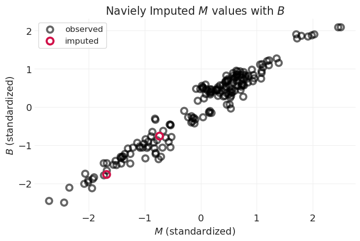
../_images/a4de3f54c84e84f5b6e4e2961542aadc23823f1cdf52ab817c063fc71fc60893.png

由于 \(M\) 与 \(B\) 强相关，因此插补的 \(M\) 值遵循线性关系

plot_posterior_imputation(
    "M", "G", naive_imputation_inference, impute_y=True, title="Naively Imputed $M$ values with $G$"
)

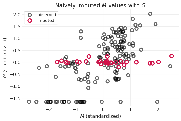
../_images/ede8d395d84c33a6433d56143d9a513aadfd861e7558e6b5cb167db092764ed2.png

由于 \(M\) 和 \(G\) 之间的关联未建模，因此插补值不遵循 \(M\) 和 \(G\) 之间的线性趋势
我们遗漏了一些信息；这是忽略完整生成模型的结果

用于比较的完整案例模型#

在这里，我们将拟合一个仅限完整案例的模型，其中不需要插补，但我们丢弃了数据。

# Complete Case
PRIMATES_CC = PRIMATES301.query(
    "brain.notnull() and body.notnull() and group_size.notnull()", engine="python"
)

G_CC = utils.standardize(np.log(PRIMATES_CC.group_size.values))
M_CC = utils.standardize(np.log(PRIMATES_CC.body.values))
B_CC = utils.standardize(np.log(PRIMATES_CC.brain.values))

# Get complete case distance matrix
PRIMATES_DISTANCE_MATRIX_CC = utils.load_data("Primates301_distance_matrix").values

# Filter out incomplete cases
PRIMATES_DISTANCE_MATRIX_CC = PRIMATES_DISTANCE_MATRIX_CC[PRIMATES_CC.index][:, PRIMATES_CC.index]

# Rescale distances to [0, 1]
D_mat_CC = PRIMATES_DISTANCE_MATRIX_CC / PRIMATES_DISTANCE_MATRIX_CC.max()
assert D_mat_CC.max() == 1

以下是使用 PyMC 的高斯过程模块的实现。

# with pm.Model() as complete_case_model:

#     # Priors
#     alpha = pm.Normal("alpha", 0, 1)
#     beta_G = pm.Normal("beta_GB", 0, 0.5)
#     beta_M = pm.Normal("beta_MB", 0, 0.5)
#     sigma = pm.Exponential("sigma", 1)

#     # Phylogenetic distance covariance
#     mean_func = MeanBodyMassSocialGroupSize(alpha, beta_G, beta_M, G_CC, M_CC)

#     # Phylogenetic distance covariance prior, L1-kernel function
#     eta_squared = pm.TruncatedNormal("eta_squared", 1, .25, lower=.01)
#     rho = pm.TruncatedNormal("rho", 3, .25, lower=.01)
#     cov_func = eta_squared * pm.gp.cov.Exponential(1, ls=rho)

#     gp = pm.gp.Marginal(mean_func=mean_func, cov_func=cov_func)
#     gp.marginal_likelihood("B", X=D_mat_CC, y=B_CC, noise=sigma)

#     complete_case_inference = pm.sample(target_accept=.95)

以下是另一种实现，它手动构建协方差函数，并将数据集直接建模为 MVNormal，其均值是 \(G\) 和 \(M\) 的线性函数，协方差由核定义。我发现这些 MVNormal 实现与讲座中的结果更吻合。

with pm.Model() as complete_case_model:

    # Priors
    alpha = pm.Normal("alpha", 0, 1)
    beta_G = pm.Normal("beta_G", 0, 0.5)
    beta_M = pm.Normal("beta_M", 0, 0.5)

    # Phylogenetic distance covariance
    eta_squared = pm.TruncatedNormal("eta_squared", 1, 0.25, lower=0.001)
    rho = pm.TruncatedNormal("rho", 3, 0.25, lower=0.001)

    K = pm.Deterministic(
        "K", generate_L1_kernel_matrix(D_mat_CC, eta_squared, rho, smoothing=0.001)
    )
    # K = pm.Deterministic('K', eta_squared * pm.math.exp(-rho * D_mat_CC))

    # Likelihood
    mu = alpha + beta_G * G_CC + beta_M * M_CC
    pm.MvNormal("B", mu=mu, cov=K, observed=B_CC)
    complete_case_inference = pm.sample()

Initializing NUTS using jitter+adapt_diag...
Multiprocess sampling (4 chains in 4 jobs)
NUTS: [alpha, beta_G, beta_M, eta_squared, rho]

Sampling 4 chains for 1_000 tune and 1_000 draw iterations (4_000 + 4_000 draws total) took 27 seconds.

比较朴素插补模型和完整案例模型的后验分布#

az.plot_dist(complete_case_inference.posterior["beta_G"], label="complete case", color="k")
az.plot_dist(naive_imputation_inference.posterior["beta_G"], label="imputed", color="C0")
plt.axvline(0, linestyle="--", color="k", label="no effect")
plt.xlabel("effect of Social Group size on Brain size, $\\beta_G$")
plt.ylabel("density")
plt.legend();

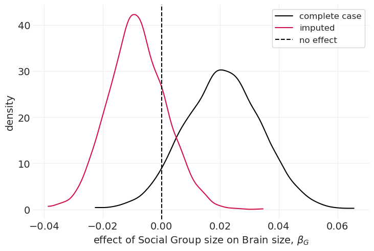
../_images/90d0b5b0d3b4dcdae2eaf38d0f987cbdd5ae91f94e64522858bedb983a55d3e9.png

我们可以看到，插补模型的后验分布减弱了群体大小对大脑大小的影响

3. 使用 \(G\) 特定的子模型插补 \(G\)#

添加群体大小的生成模型。但是，再说一次，我们将分小步进行，缓慢构建复杂性

仅对体重对群体大小的影响建模的模型 \(M \rightarrow G\)
仅包括社会群体系统发育相互作用的模型
结合系统发育和 \(M \rightarrow G\) 的模型

1. 仅对体重对群体大小的影响建模的模型 \(M \rightarrow G\)#

以下是使用 PyMC 的高斯过程模块的实现。

# PRIMATE_ID, PRIMATE = pd.factorize(PRIMATES['name'].values)
# coords = {'primate': PRIMATE}

# with pm.Model(coords=coords) as G_body_mass_model:

#     # Priors
#     alpha_G = pm.Normal("alpha_G", 0, 1)
#     beta_MG = pm.Normal("beta_MG", 0, 0.5)
#     sigma_G = pm.Exponential("sigma_G", 1)

#     alpha_B = pm.Normal("alpha_B", 0, 1)
#     beta_GB = pm.Normal("beta_GB", 0, 0.5)
#     beta_MB = pm.Normal("beta_MB", 0, 0.5)
#     sigma_B = pm.Exponential("sigma_B", 1)

#     # Naive imputation for M
#     M = pm.Normal("M", 0, 1, observed=M_obs, dims='primate')

#     # G model M->G (performs imputation)
#     mu_G = alpha_G + beta_MG * M
#     G = pm.Normal("G", mu_G, sigma_G, observed=G_obs)

#     # B Model
#     eta_squared_B = pm.TruncatedNormal("eta_squared_B", 1, .25, lower=.01)
#     rho_B = pm.TruncatedNormal("rho_B", 3, .25, lower=.01)
#     cov_func_B = eta_squared_B * pm.gp.cov.Exponential(1, ls=rho_B)
#     mean_func_B = MeanBodyMassSocialGroupSize(alpha_B, beta_GB, beta_MB, G, M)

#     # Gaussian Process
#     gp_B = pm.gp.Marginal(mean_func=mean_func_B, cov_func=cov_func_B)
#     gp_B.marginal_likelihood("B", X=D_mat, y=B_obs, noise=sigma_B)

#     G_body_mass_inference = pm.sample(target_accept=.95, cores=1)

以下是另一种实现，它手动构建协方差函数，并将数据集直接建模为 MVNormal，其均值是 \(G\) 和 \(M\) 的线性函数，协方差由核定义。我发现这些 MVNormal 实现与讲座中的结果更吻合。

PRIMATE_ID, PRIMATE = pd.factorize(PRIMATES["name"].values)
coords = {"primate": PRIMATE}

with pm.Model(coords=coords) as G_body_mass_model:

    # Priors
    alpha_B = pm.Normal("alpha_B", 0, 1)
    beta_GB = pm.Normal("beta_GB", 0, 0.5)
    beta_MB = pm.Normal("beta_MB", 0, 0.5)

    alpha_G = pm.Normal("alpha_G", 0, 1)
    beta_MG = pm.Normal("beta_MG", 0, 0.5)
    sigma_G = pm.Exponential("sigma_G", 1)

    # Naive imputation for M
    M = pm.Normal("M", 0, 1, observed=M_obs, dims="primate")

    # Body-mass only, no interactions
    mu_G = alpha_G + beta_MG * M
    G = pm.Normal("G", mu_G, sigma_G, observed=G_obs)

    # B Model
    eta_squared_B = pm.TruncatedNormal("eta_squared_B", 1, 0.25, lower=0.001)
    rho_B = pm.TruncatedNormal("rho_B", 3, 0.25, lower=0.001)
    K_B = pm.Deterministic("K_B", eta_squared_B * pm.math.exp(-rho_B * D_mat))

    # Likelihood for B
    mu_B = alpha_B + beta_GB * G + beta_MB * M
    pm.MvNormal("B", mu=mu_B, cov=K_B, observed=B_obs)

    G_body_mass_inference = pm.sample()

Initializing NUTS using jitter+adapt_diag...
Multiprocess sampling (4 chains in 4 jobs)
NUTS: [alpha_B, beta_GB, beta_MB, alpha_G, beta_MG, sigma_G, M_unobserved, G_unobserved, eta_squared_B, rho_B]

Sampling 4 chains for 1_000 tune and 1_000 draw iterations (4_000 + 4_000 draws total) took 103 seconds.

查看仅限 \(M \rightarrow G\) 的插补#

plot_posterior_imputation(
    "M", "G", G_body_mass_inference, impute_y=True, title="$M \\rightarrow G$ model"
)

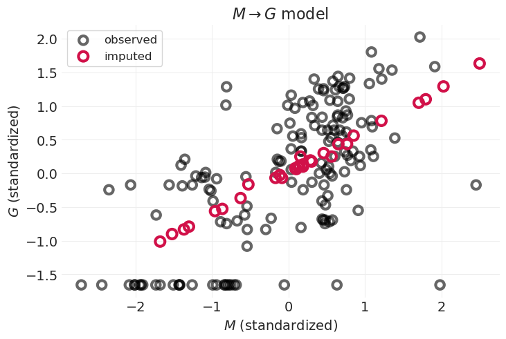
../_images/f47951d1436c94d90c98a0d7ac378c0b0aba37ca8dbf0c16f7f118ffd2d777e5.png

通过对 \(M\) 对 \(G\) 的影响进行建模，我们能够捕获线性趋势；插补变量沿此趋势线分布
但是，通过忽略系统发育相似性，我们无法捕获数据中的非线性
- 例如，一些群体大小较小的物种位于图的左下方，不遵循线性趋势

2. 仅包括社会群体系统发育相互作用的模型#

以下是使用 PyMC 的高斯过程模块的实现。

# PRIMATE_ID, PRIMATE = pd.factorize(PRIMATES['name'].values)
# coords = {'primate': PRIMATE}

# with pm.Model(coords=coords) as G_phylogeny_model:

#     # Priors
#     alpha_G = pm.Normal("alpha_G", 0, 1)
#     sigma_G = pm.Exponential("sigma_G", 1)

#     alpha_B = pm.Normal("alpha_B", 0, 1)
#     beta_GB = pm.Normal("beta_GB", 0, 0.5)
#     beta_MB = pm.Normal("beta_MB", 0, 0.5)
#     sigma_B = pm.Exponential("sigma_B", 1)

#     # Naive imputation for M
#     M = pm.Normal("M", 0, 1, observed=M_obs, dims='primate')

#     # G model, interactions only
#     mean_func_G = MeanBodyMassSocialGroupSize(alpha_G, 0, 0, 0, 0)

#     eta_squared_G = pm.TruncatedNormal("eta_squared_G", 1, .25, lower=.01)
#     rho_G = pm.TruncatedNormal("rho_G", 3, .25, lower=.01)
#     cov_func_G = eta_squared_G * pm.gp.cov.Exponential(1, ls=rho_G)

#     gp_G = pm.gp.Marginal(mean_func=mean_func_G, cov_func=cov_func_G)
#     G = gp_G.marginal_likelihood("G", X=D_mat, y=G_obs, noise=sigma_G)

#     # B Model
#     mean_func_B = MeanBodyMassSocialGroupSize(alpha_B, beta_GB, beta_MB, G, M)

#     eta_squared_B = pm.TruncatedNormal("eta_squared_B", 1, .25, lower=.01)
#     rho_B = pm.TruncatedNormal("rho_B", 3, .25, lower=.01)
#     cov_func_B = eta_squared_B * pm.gp.cov.Exponential(1, ls=rho_B)

#     gp_B = pm.gp.Marginal(mean_func=mean_func_B, cov_func=cov_func_B)
#     gp_B.marginal_likelihood("B", X=D_mat, y=B_obs, noise=sigma_B)

#     G_phylogeny_inference = pm.sample(target_accept=.95, cores=1)

以下是另一种实现，它手动构建协方差函数，并将数据集直接建模为 MVNormal，其均值是 \(G\) 和 \(M\) 的线性函数，协方差由核定义。我发现这些 MVNormal 实现与讲座中的结果更吻合。

coords = {"primate": PRIMATES["name"].values}
with pm.Model(coords=coords) as G_phylogeny_model:

    # Priors
    alpha_B = pm.Normal("alpha_B", 0, 1)
    beta_GB = pm.Normal("beta_GB", 0, 0.5)
    beta_MB = pm.Normal("beta_MB", 0, 0.5)

    alpha_G = pm.Normal("alpha_G", 0, 1)
    beta_MG = pm.Normal("beta_MG", 0, 0.5)

    # Naive imputation for M
    M = pm.Normal("M", 0, 1, observed=M_obs, dims="primate")

    # G Model Imputation, only phylogenetic interaction
    eta_squared_G = pm.TruncatedNormal("eta_squared_G", 1, 0.25, lower=0.001)
    rho_G = pm.TruncatedNormal("rho_G", 3, 0.25, lower=0.001)
    K_G = pm.Deterministic("K_G", eta_squared_G * pm.math.exp(-rho_G * D_mat))

    mu_G = pm.math.zeros_like(B_obs)  # no linear model
    G = pm.MvNormal("G", mu=mu_G, cov=K_G, observed=G_obs)

    # B Model
    eta_squared_B = pm.TruncatedNormal("eta_squared_B", 1, 0.25, lower=0.001)
    rho_B = pm.TruncatedNormal("rho_B", 3, 0.25, lower=0.001)
    K_B = pm.Deterministic("K_B", eta_squared_B * pm.math.exp(-rho_B * D_mat))

    # Likelihood for B
    mu_B = alpha_B + beta_GB * G + beta_MB * M
    pm.MvNormal("B", mu=mu_B, cov=K_B, observed=B_obs)

    G_phylogeny_inference = pm.sample()

Initializing NUTS using jitter+adapt_diag...
Multiprocess sampling (4 chains in 4 jobs)
NUTS: [alpha_B, beta_GB, beta_MB, alpha_G, beta_MG, M_unobserved, eta_squared_G, rho_G, G_unobserved, eta_squared_B, rho_B]

Sampling 4 chains for 1_000 tune and 1_000 draw iterations (4_000 + 4_000 draws total) took 200 seconds.

查看仅限系统发育的插补#

plot_posterior_imputation(
    "M", "G", G_phylogeny_inference, impute_y=True, impute_color="C1", title="Phylogeny-only Model"
)

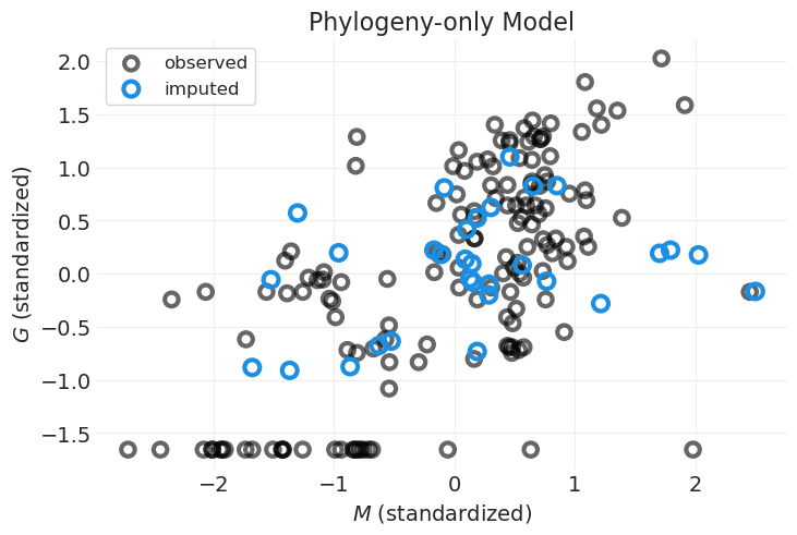
../_images/7fa4f006b711230c465e20fa9444c2e231678c0fb14bbe16ddaa313ceca8caab.png

⚠️ 由于某些原因，在尝试了 PyMC 的 gp 模块的两种不同实现以及使用 MVNormal 似然函数（两者都给出相似的结果）后，我无法复制讲座中介绍的针对独居灵长类动物的插补。

欢迎就我可能在这里做错的事情提出意见和建议

3. 拟合结合系统发育和 \(M \rightarrow G\) 的模型#

以下是使用 PyMC 的高斯过程模块实现模型的实现。

# PRIMATE_ID, PRIMATE = pd.factorize(PRIMATES['name'].values)
# coords = {'primate': PRIMATE}

# with pm.Model(coords=coords) as G_imputation_model:

#     # Priors
#     alpha_G = pm.Normal("alpha_G", 0, 1)
#     beta_MG = pm.Normal("beta_MG", 0, 1)
#     sigma_G = pm.Exponential("sigma_G", 1)

#     alpha_B = pm.Normal("alpha_B", 0, 1)
#     beta_GB = pm.Normal("beta_GB", 0, 0.5)
#     beta_MB = pm.Normal("beta_MB", 0, 0.5)
#     sigma_B = pm.Exponential("sigma_B", 1)

#     # Naive imputation for M
#     M = pm.Normal("M", 0, 1, observed=M_obs, dims='primate')

#     # G model, interactions only
#     mean_func_G = MeanBodyMassSocialGroupSize(alpha_G, 0, beta_MG, 0, M)

#     eta_squared_G = pm.TruncatedNormal("eta_squared_G", 1, .25, lower=.01)
#     rho_G = pm.TruncatedNormal("rho_G", 3, .25, lower=.01)
#     cov_func_G = eta_squared_G * pm.gp.cov.Exponential(1, ls=rho_G)

#     gp_G = pm.gp.Marginal(mean_func=mean_func_G, cov_func=cov_func_G)
#     G = gp_G.marginal_likelihood("G", X=D_mat, y=G_obs, noise=sigma_G)

#     # B Model
#     mean_func_B = MeanBodyMassSocialGroupSize(alpha_B, beta_GB, beta_MB, G, M)

#     eta_squared_B = pm.TruncatedNormal("eta_squared_B", 1, .25, lower=.01)
#     rho_B = pm.TruncatedNormal("rho_B", 3, .25, lower=.01)
#     cov_func_B = eta_squared_B * pm.gp.cov.Exponential(1, ls=rho_B)

#     gp_B = pm.gp.Marginal(mean_func=mean_func_B, cov_func=cov_func_B)
#     gp_B.marginal_likelihood("B", X=D_mat, y=B_obs, noise=sigma_B)

#     G_imputation_inference = pm.sample(target_accept=.95, cores=1)

以下是另一种实现，它手动构建协方差函数，并将数据集直接建模为 MVNormal，其均值是 \(G\) 和 \(M\) 的线性函数，协方差由核定义。我发现这些 MVNormal 实现与讲座中的结果更吻合。

coords = {"primate": PRIMATES["name"].values}
with pm.Model(coords=coords) as G_imputation_model:

    # Priors
    alpha_B = pm.Normal("alpha_B", 0, 1)
    beta_GB = pm.Normal("beta_GB", 0, 0.5)
    beta_MB = pm.Normal("beta_MB", 0, 0.5)

    alpha_G = pm.Normal("alpha_G", 0, 1)
    beta_MG = pm.Normal("beta_MG", 0, 0.5)

    # Naive imputation for M
    M = pm.Normal("M", 0, 1, observed=M_obs, dims="primate")

    # G Model Imputation
    eta_squared_G = pm.TruncatedNormal("eta_squared_G", 1, 0.25, lower=0.001)
    rho_G = pm.TruncatedNormal("rho_G", 3, 0.25, lower=0.001)

    K_G = pm.Deterministic("K_G", eta_squared_G * pm.math.exp(-rho_G * D_mat))
    mu_G = alpha_G + beta_MG * M
    G = pm.MvNormal("G", mu=mu_G, cov=K_G, observed=G_obs)

    # B Model
    eta_squared_B = pm.TruncatedNormal("eta_squared_B", 1, 0.25, lower=0.001)
    rho_B = pm.TruncatedNormal("rho_B", 3, 0.25, lower=0.001)
    K_B = pm.Deterministic("K_B", eta_squared_B * pm.math.exp(-rho_B * D_mat))

    # Likelihood for B
    mu_B = alpha_B + beta_GB * G + beta_MB * M
    pm.MvNormal("B", mu=mu_B, cov=K_B, observed=B_obs)

    G_imputation_inference = pm.sample()

Initializing NUTS using jitter+adapt_diag...
Multiprocess sampling (4 chains in 4 jobs)
NUTS: [alpha_B, beta_GB, beta_MB, alpha_G, beta_MG, M_unobserved, eta_squared_G, rho_G, G_unobserved, eta_squared_B, rho_B]

Sampling 4 chains for 1_000 tune and 1_000 draw iterations (4_000 + 4_000 draws total) took 193 seconds.

plot_posterior_imputation(
    "M",
    "G",
    G_imputation_inference,
    impute_y=True,
    impute_color="C4",
    title="Phylogeny + $M \\rightarrow G$ model",
)

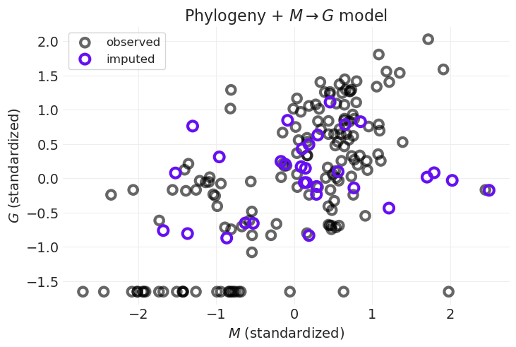
../_images/45b4f3d9989e7b32fc74cbf46d0f6558cce3f8ac4a11673e0f1ad2f41121d09a.png

紫色点向回归线移动

⚠️ 由于某些原因，在尝试了 PyMC 的 gp 模块的两种不同实现以及使用 MVNormal 似然函数（两者都给出相似的结果）后，我无法复制讲座中介绍的针对独居灵长类动物的插补。

欢迎就我可能在这里做错的事情提出意见和建议

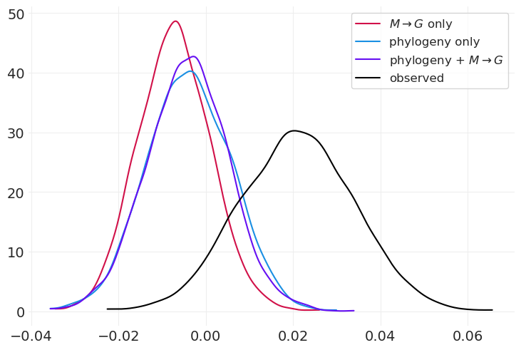
az.plot_dist(
    G_body_mass_inference.posterior["beta_GB"], color="C0", label="$M \\rightarrow G$ only"
)
az.plot_dist(G_phylogeny_inference.posterior["beta_GB"], color="C1", label="phylogeny only")
az.plot_dist(
    G_imputation_inference.posterior["beta_GB"], color="C4", label="phylogeny + $M \\rightarrow G$"
)
az.plot_dist(complete_case_inference.posterior["beta_G"], color="k", label="observed");

../_images/50392f91bbb4037c23fd70bafd5bc58533c0a2331cbb0aeb2dd2ea3d5b835bb0.png

4. 使用每个子模型插补 \(B,G,M\)#

以下是使用 PyMC 的高斯过程模块的实现。

# with pm.Model() as full_model:

#     # Priors
#     sigma_M = pm.Exponential("sigma_M", 1

#     alpha_G = pm.Normal("alpha_G", 0, 1)
#     beta_MG = pm.Normal("beta_MG", 0, 1)
#     sigma_G = pm.Exponential("sigma_G", 1)

#     alpha_B = pm.Normal("alpha_B", 0, 1)
#     beta_GB = pm.Normal("beta_GB", 0, 0.5)
#     beta_MB = pm.Normal("beta_MB", 0, 0.5)
#     sigma_B = pm.Exponential("sigma_B", 1))

#     # Naive imputation for M
#     eta_squared_M = pm.TruncatedNormal("eta_squared_M", 1, .25, lower=.01)
#     rho_M = pm.TruncatedNormal("rho_M", 3, .25, lower=.01)

#     cov_func_M = eta_squared_M * pm.gp.cov.Exponential(1, ls=rho_M)
#     mean_func_M = pm.gp.mean.Zero()

#     gp_M = pm.gp.Marginal(mean_func=mean_func_M, cov_func=cov_func_M)
#     M = gp_M.marginal_likelihood("M", X=D_mat, y=M_obs, noise=sigma_M)

#     # G model, interactions only
#     mean_func_G = MeanBodyMassSocialGroupSize(alpha_G, 0, beta_MG, 0, M)

#     eta_squared_G = pm.TruncatedNormal("eta_squared_G", 1, .25, lower=.01)
#     rho_G = pm.TruncatedNormal("rho_G", 3, .25, lower=.01)
#     cov_func_G = eta_squared_G * pm.gp.cov.Exponential(1, ls=rho_G)

#     gp_G = pm.gp.Marginal(mean_func=mean_func_G, cov_func=cov_func_G)
#     G = gp_G.marginal_likelihood("G", X=D_mat, y=G_obs, noise=sigma_G)

#     # B Model
#     mean_func_B = MeanBodyMassSocialGroupSize(alpha_B, beta_GB, beta_MB, G, M)

#     eta_squared_B = pm.TruncatedNormal("eta_squared_B", 1, .25, lower=.01)
#     rho_B = pm.TruncatedNormal("rho_B", 3, .25, lower=.01)
#     cov_func_B = eta_squared_B * pm.gp.cov.Exponential(1, ls=rho_B)

#     gp_B = pm.gp.Marginal(mean_func=mean_func_B, cov_func=cov_func_B)
#     gp_B.marginal_likelihood("B", X=D_mat, y=B_obs, noise=sigma_B)

#     full_inference = pm.sample(target_accept=.95, cores=1)

以下是另一种实现，它手动构建协方差函数，并将数据集直接建模为 MVNormal，其均值是 \(G\) 和 \(M\) 的线性函数，协方差由核定义。我发现这些 MVNormal 实现与讲座中的结果更吻合。

coords = {"primate": PRIMATES["name"].values}
with pm.Model(coords=coords) as full_model:

    # Priors
    alpha_B = pm.Normal("alpha_B", 0, 1)
    beta_GB = pm.Normal("beta_GB", 0, 0.5)
    beta_MB = pm.Normal("beta_MB", 0, 0.5)

    alpha_G = pm.Normal("alpha_G", 0, 1)
    beta_MG = pm.Normal("beta_MG", 0, 0.5)

    # M model (imputation)
    eta_squared_M = pm.TruncatedNormal("eta_squared_M", 1, 0.25, lower=0.001)
    rho_M = pm.TruncatedNormal("rho_M", 3, 0.25, lower=0.001)

    K_M = pm.Deterministic("K_M", eta_squared_M * pm.math.exp(-rho_M * D_mat))
    mu_M = pm.math.zeros_like(M_obs)
    M = pm.MvNormal("M", mu=mu_M, cov=K_M, observed=M_obs)

    # G Model (imputation)
    eta_squared_G = pm.TruncatedNormal("eta_squared_G", 1, 0.25, lower=0.001)
    rho_G = pm.TruncatedNormal("rho_G", 3, 0.25, lower=0.001)

    K_G = pm.Deterministic("K_G", eta_squared_G * pm.math.exp(-rho_G * D_mat))
    mu_G = alpha_G + beta_MG * M
    G = pm.MvNormal("G", mu=mu_G, cov=K_G, observed=G_obs)

    # B Model
    eta_squared_B = pm.TruncatedNormal("eta_squared_B", 1, 0.25, lower=0.001)
    rho_B = pm.TruncatedNormal("rho_B", 3, 0.25, lower=0.001)
    K_B = pm.Deterministic("K_B", eta_squared_B * pm.math.exp(-rho_B * D_mat))

    # Likelihood for B
    mu_B = alpha_B + beta_GB * G + beta_MB * M
    pm.MvNormal("B", mu=mu_B, cov=K_B, observed=B_obs)

    full_inference = pm.sample(nuts_sampler="nutpie")

采样器进度

总链数：4

活跃链数：0

已完成链数：4

采样 3 分钟

预计完成时间：现在

抽取	步长	梯度/抽取
2000	0.58	7
2000	0.61	7
2000	0.59	7
2000	0.59	7

plot_posterior_imputation(
    "M", "G", full_inference, impute_y=True, impute_color="C5", title="Full model, including M"
)

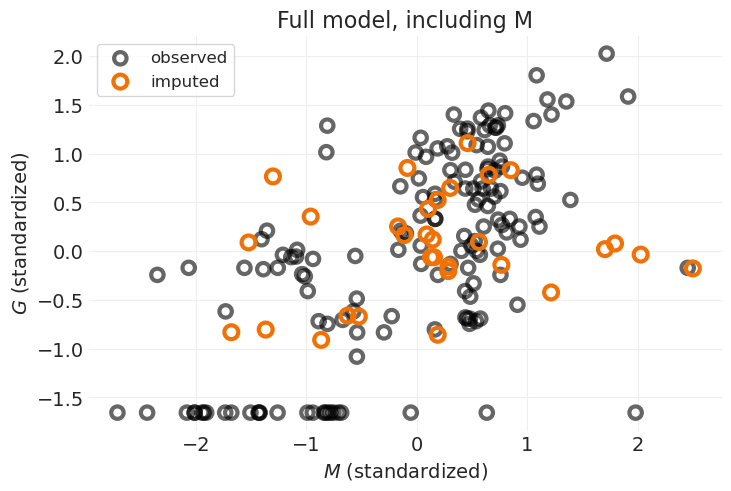
../_images/2bc66172483f70b571f2739ada187348ede3332c0c65e80b00dfd614b7205774.png

插补与之前的模型相比变化不大，之前的模型没有直接对 \(M\) 的原因进行建模。我认为这是因为只有两个缺失的 \(M\) 值

az.plot_dist(
    G_body_mass_inference.posterior["beta_GB"], color="C0", label="$M \\rightarrow G$ only"
)
az.plot_dist(G_phylogeny_inference.posterior["beta_GB"], color="C1", label="phylogeny only")
az.plot_dist(
    G_imputation_inference.posterior["beta_GB"], color="C4", label="phylogeny + $M \\rightarrow G$"
)
az.plot_dist(full_inference.posterior["beta_GB"], color="C5", label="full model, including M")
az.plot_dist(complete_case_inference.posterior["beta_G"], color="k", label="observed");

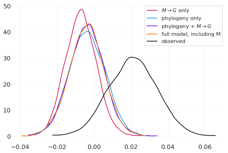
../_images/bd2b2db66556f41fb3c4cc8512a37e0d25ee7a86f7b6ed1a4497154c8844c8f1.png

我们还获得了与系统发育 + \(M \rightarrow G\) 模型非常相似的效果

回顾：插补灵长类动物#

核心思想：缺失值具有概率分布
像图形一样思考，而不是像回归一样思考
在预测变量之间没有关系的情况下盲目插补可能存在风险
- 利用部分合并
即使插补不会改变结果，这也是科学责任

作者#

移植到 PyMC：Dustin Stansbury (2024)
基于 Richard McElreath 的 Statistical Rethinking (2023) 讲座

%load_ext watermark
%watermark -n -u -v -iv -w -p pytensor,xarray

Last updated: Tue Dec 17 2024

Python implementation: CPython
Python version       : 3.12.5
IPython version      : 8.27.0

pytensor: 2.26.4
xarray  : 2024.7.0

matplotlib : 3.9.2
arviz      : 0.19.0
xarray     : 2024.7.0
pymc       : 5.19.1
scipy      : 1.14.1
statsmodels: 0.14.2
numpy      : 1.26.4
pandas     : 2.2.2

Watermark: 2.5.0

许可证声明#

此示例画廊中的所有 notebook 均根据 MIT 许可证提供，该许可证允许修改和再分发以用于任何用途，前提是保留版权和许可证声明。

引用 PyMC 示例#

要引用此 notebook，请使用 Zenodo 为 pymc-examples 存储库提供的 DOI。

重要提示

许多 notebook 都改编自其他来源：博客、书籍……在这种情况下，您也应该引用原始来源。

另请记住引用您的代码使用的相关库。

这是一个 bibtex 中的引用模板

@incollection{citekey,
  author    = "<notebook authors, see above>",
  title     = "<notebook title>",
  editor    = "PyMC Team",
  booktitle = "PyMC examples",
  doi       = "10.5281/zenodo.5654871"
}

一旦渲染，它可能看起来像

分类

标签

缺失数据#

缺失数据，已找到#

处理缺失数据是一个工作流程#

如何处理缺失数据？#

狗吃了我的作业：查看不同的缺失数据情景#

狗通常是良性的#

模拟随机吃作业#

狗根据家庭作业的原因（学生能力）吃家庭作业#

模拟治疗效果线性影响结果的数据#

模拟治疗效果非线性影响结果的数据#

狗根据家庭作业状态本身来吃家庭作业#

模拟一些线性数据#

典型案例#

贝叶斯插补#

插补或边缘化#

何时插补？何时边缘化？#

重新审视系统发育回归#

插补灵长类动物#

重新审视之前的因果模型#

现在让我们包括缺失值可能如何发生#

关于是什么导致数据缺失的一些假设…#

同时为多个变量建模缺失数据#

\(M, G, B\) 都具有缺失值 \(M^*, G^*, B^*\)#

处理大脑大小 \(B\) 中的缺失值#

大脑大小 \(B\) 模型#

群体大小 \(G\) 模型#

体重 \(M\) 模型#

绘制缺失的猫头鹰 🦉#

1. 忽略缺少 \(B\) 值的案例#

筛选掉缺少大脑体积测量的观测值#

在结果数据集上交叉制表 \(G,M\) 的缺失情况#

2. 天真地插补 \(G,M\)，忽略每个模型的模型#

拟合忽略 \(G,M\) 子模型的插补模型#

加载系统发育距离矩阵#

拟合朴素插补模型#

演示插补的效果#

\(M\) 插补#

\(M\) 的先验值#

\(G\) 插补#

\(G\) 的先验值#

绘制后验插补图#

查看插补值#

用于比较的完整案例模型#

比较朴素插补模型和完整案例模型的后验分布#

3. 使用 \(G\) 特定的子模型插补 \(G\)#

1. 仅对体重对群体大小的影响建模的模型 \(M \rightarrow G\)#

查看仅限 \(M \rightarrow G\) 的插补#

2. 仅包括社会群体系统发育相互作用的模型#

查看仅限系统发育的插补#

3. 拟合结合系统发育和 \(M \rightarrow G\) 的模型#

4. 使用每个子模型插补 \(B,G,M\)#

回顾：插补灵长类动物#

作者#

许可证声明#

引用 PyMC 示例#

\(M, G, B\) 都具有缺失值 \(M^, G^, B^*\)#