


广义线性疯狂#
此笔记本是 PyMC 对 Richard McElreath 的 Statistical Rethinking 2023 系列讲座的移植。
视频 - 第 19 讲 - 广义线性疯狂# 第 19 讲 - 广义线性疯狂
# Ignore warnings
import warnings

import arviz as az
import numpy as np
import pandas as pd
import pymc as pm
import statsmodels.formula.api as smf
import utils as utils
import xarray as xr

from matplotlib import pyplot as plt
from matplotlib import style
from scipy import stats as stats

warnings.filterwarnings("ignore")

# Set matplotlib style
STYLE = "statistical-rethinking-2023.mplstyle"
style.use(STYLE)
GLM、GLMM 和广义线性习惯#
灵活的关联引擎,而不是生成现象的机制的机械科学模型
可能遗漏信息
可能效率较低
机械因果模型通常更易于解释
相反,它们是信息论设备
即便如此,超过 90% 的科学工作是使用 GLM/GLMM 完成的
替代方法 - 从简单的科学原理开始,并构建估计
重新审视人体身高建模 ⚖️#
人的体重与人的体积成正比
较高的人比矮小的人体积更大
因此,较高的人体重更重(我知道这非常基础,但这正是重点)
因此,人的体重归根结底是简单的物理学:人的形状决定了其质量,从而决定了其体重
我们可以用多种方式对人的形状进行建模,但最简单(尽管是卡通化)的方式可能是圆柱体。
人很少比他们高更宽——我们可以将圆柱体的半径建模为身高的比例
尽可能将统计估计推到分析流程的下游
卡通化科学模型#
捕捉身高和体重之间的因果关系
因果关系是因为,它告诉我们改变身高将如何影响体重
\(W\) 体重(观测数据,类似于 Howell 数据集)
\(h\) heith (observed data)
\(k\) 密度(要估计的参数)
\(p\) 身高比例(要估计的参数)
统计模型#
科学模型到统计模型的一般转换#
先验#
现在参数 \(p,k\) 具有现实世界的解释,确定它们的先验比典型的 GLM/GLMM 更直接
先验开发工作流程
选择测量尺度(或移除它们)
模拟
思考
1. 测量尺度
\(\mu\) - \(kg\)
\(H\) - \(cm^3\)
\(k\) - \(kg/cm^3\)
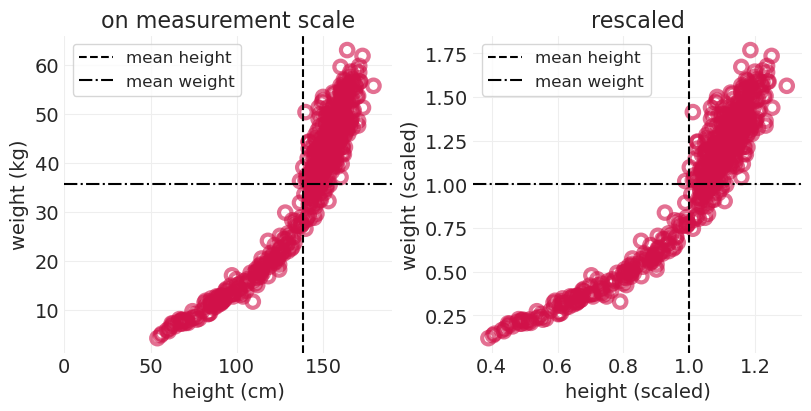
你总是可以使用参考重新缩放测量尺度
例如,除以平均体重和身高
尽可能尝试除掉测量单位
通常更容易处理无量纲量
HOWELL = utils.load_data("Howell1")

# Add rescaled data
HOWELL.loc[:, "height_scaled"] = HOWELL.height / HOWELL.height.mean()
HOWELL.loc[:, "weight_scaled"] = HOWELL.weight / HOWELL.weight.mean()
HOWELL
| 身高 | 体重 | 年龄 | 男性 | 身高_缩放 | 体重_缩放 | |
|---|---|---|---|---|---|---|
| 0 | 151.765 | 47.825606 | 63.0 | 1 | 1.097650 | 1.343015 |
| 1 | 139.700 | 36.485807 | 63.0 | 0 | 1.010389 | 1.024577 |
| 2 | 136.525 | 31.864838 | 65.0 | 0 | 0.987425 | 0.894813 |
| 3 | 156.845 | 53.041914 | 41.0 | 1 | 1.134391 | 1.489497 |
| 4 | 145.415 | 41.276872 | 51.0 | 0 | 1.051723 | 1.159117 |
| ... | ... | ... | ... | ... | ... | ... |
| 539 | 145.415 | 31.127751 | 17.0 | 1 | 1.051723 | 0.874114 |
| 540 | 162.560 | 52.163080 | 31.0 | 1 | 1.175725 | 1.464818 |
| 541 | 156.210 | 54.062497 | 21.0 | 0 | 1.129798 | 1.518157 |
| 542 | 71.120 | 8.051258 | 0.0 | 1 | 0.514380 | 0.226092 |
| 543 | 158.750 | 52.531624 | 68.0 | 1 | 1.148169 | 1.475167 |
544 行 × 6 列
_, axs = plt.subplots(1, 2, figsize=(8, 4))

plt.sca(axs[0])
utils.plot_scatter(HOWELL.height, HOWELL.weight)
plt.axvline(HOWELL.height.mean(), color="k", linestyle="--", label="mean height")
plt.axhline(HOWELL.weight.mean(), color="k", linestyle="-.", label="mean weight")
plt.xlim([0, 190])
plt.xlabel("height (cm)")
plt.ylabel("weight (kg)")
plt.legend()
plt.title("on measurement scale")

plt.sca(axs[1])
utils.plot_scatter(HOWELL.height_scaled, HOWELL.weight_scaled)
plt.axvline(HOWELL.height_scaled.mean(), color="k", linestyle="--", label="mean height")
plt.axhline(HOWELL.weight_scaled.mean(), color="k", linestyle="-.", label="mean weight")
plt.xlabel("height (scaled)")
plt.ylabel("weight (scaled)")
plt.legend()
plt.title("rescaled");
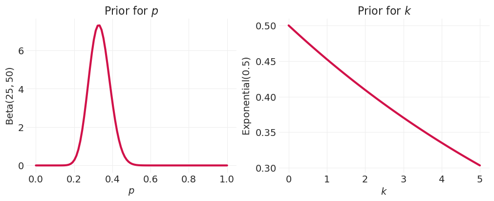
2. 模拟
比例,\(p\)
根据比例的定义 \(\in (0, 1)\)
必须 \(\lt 0.5\) 因为人类通常不会比他们高更宽
密度,\(k\)
密度必须 \(\gt 1\) 因为身高和体重之间存在正相关关系
p_prior = stats.beta(a=25, b=50)
ps = np.linspace(0, 1, 100)

rate = 0.5
k_prior = stats.expon(scale=1 / rate)
ks = np.linspace(0, 5, 100)


_, axs = plt.subplots(1, 2, figsize=(10, 4))

plt.sca(axs[0])
utils.plot_line(ps, p_prior.pdf(ps), label=None)
plt.xlabel("$p$")
plt.ylabel("Beta$(25, 50)$")
plt.title("Prior for $p$")


plt.sca(axs[1])
utils.plot_line(ks, k_prior.pdf(ps), label=None)
plt.xlabel("$k$")
plt.ylabel("Exponential$(0.5)$")
plt.title("Prior for $k$");
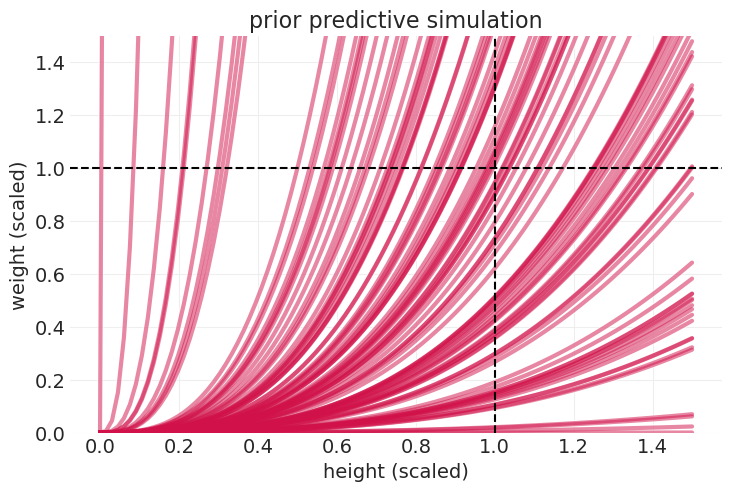
先验预测模拟#
np.random.seed(123)
n_prior_samples = 100
p_samples = p_prior.rvs(size=n_prior_samples)
k_samples = k_prior.rvs(size=n_prior_samples)
sigma_samples = stats.expon(scale=1).rvs(n_prior_samples)

heights = np.linspace(0, 1.5, 100)[:, None]

# Log-normally-distributed weight
prior_mus = np.log(np.pi * k_samples * p_samples**2 * heights**3)

# expected value on natural scale
prior_lines = np.exp(prior_mus + sigma_samples**2 / 2)

utils.plot_line(heights, prior_lines, label=None, color="C0", alpha=0.5)
plt.axvline(1, color="k", linestyle="--", zorder=100)
plt.axhline(1, color="k", linestyle="--", zorder=100)
plt.ylim([0, 1.5])
plt.xlabel("height (scaled)")
plt.ylabel("weight (scaled)")
plt.title("prior predictive simulation");
拟合统计模型#
with pm.Model() as cylinder_model:
    H = pm.Data("H", HOWELL.height_scaled, dims="obs_id")
    W = HOWELL.weight_scaled
    PI = 3.141593

    sigma = pm.Exponential("sigma", 1)
    p = pm.Beta("p", 25, 50)
    k = pm.Exponential("k", 0.5)

    mu = pm.math.log(PI * k * p**2 * H**3)
    pm.LogNormal("W", mu, sigma, observed=W, dims="obs_id")
    cylinder_inference = pm.sample()
Initializing NUTS using jitter+adapt_diag...
Multiprocess sampling (4 chains in 4 jobs)
NUTS: [sigma, p, k]
Sampling 4 chains for 1_000 tune and 1_000 draw iterations (4_000 + 4_000 draws total) took 7 seconds.
def plot_cylinder_model_posterior(model, inference, title=None):
    heights = np.linspace(0, 1.3, 100)
    with model:
        pm.set_data({"H": heights})
        ppd = pm.sample_posterior_predictive(
            inference,
            return_inferencedata=True,
            predictions=True,
            extend_inferencedata=False,
        )
    az.plot_hdi(heights, ppd.predictions["W"], color="C0")
    utils.plot_line(
        heights, ppd.predictions["W"].mean(dim=("chain", "draw")), color="k", label="posterior"
    )
    utils.plot_scatter(HOWELL.height_scaled, HOWELL.weight_scaled, color="C0")
    plt.xlabel("height (scaled)")
    plt.ylabel("weight (scaled)")
    plt.legend()
    plt.title(title)
plot_cylinder_model_posterior(cylinder_model, cylinder_inference);
Sampling: [W]
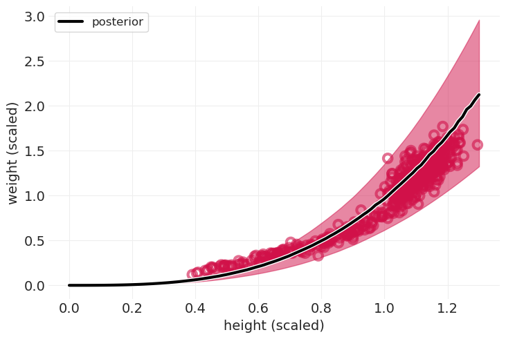
有见地的误差#
对于圆柱体来说还不错
儿童的拟合效果不佳
在科学模型中,误差是有信息的
可能 \(p\) 对儿童来说是不同的
3. 思考
贝叶斯推断发现 \(k\) 和 \(p\) 在功能上相关
您可以使用代数推导出相同的关系,并认为平均人的身高为 1
n_posterior_samples = 300
utils.plot_scatter(
    cylinder_inference.posterior["p"][0, :n_posterior_samples] ** 2,
    cylinder_inference.posterior["k"][0, :n_posterior_samples],
    label="posterior samples",
)
p_squared = np.linspace(0.03, 0.35, 100)
k_analytic = 1 / (np.pi * p_squared)

utils.plot_line(p_squared, k_analytic, color="k", label=r"$k=1/\pi p^2$")
plt.legend()
plt.xlabel("$p^2$")
plt.ylabel("$k$")
plt.title("$k$ is clearly a function of $p^2$");
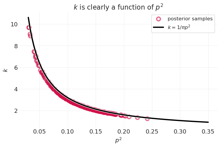
事实证明,我们甚至不需要参数 \(k, p\)。如果我们可以将模型中所有参数的乘积得到一个参数 \(\theta=kp^2\),我们可以使用相同的平均人技巧来求解上述方程
因此,参数 \(\theta = k p^2\) 只是一个常数 \(1/\pi\),所以 没有参数需要估计 🤯
拟合无量纲圆柱体模型#
with pm.Model() as dimensionless_cylinder_model:
    H = pm.Data("H", HOWELL.height_scaled, dims="obs_id")
    W = HOWELL.weight_scaled

    sigma = pm.Exponential("sigma", 1)

    mu = pm.math.log(H**3)
    pm.LogNormal("W", mu, sigma, observed=W, dims="obs_id")
    dimensionless_cylinder_inference = pm.sample()
Initializing NUTS using jitter+adapt_diag...
Multiprocess sampling (4 chains in 4 jobs)
NUTS: [sigma]
Sampling 4 chains for 1_000 tune and 1_000 draw iterations (4_000 + 4_000 draws total) took 1 seconds.
plot_cylinder_model_posterior(
    dimensionless_cylinder_model, dimensionless_cylinder_inference, title="Dimensionless Model"
);
Sampling: [W]

plot_cylinder_model_posterior(
    cylinder_model, cylinder_inference, title="Parameterized Model\n(very similar predictions)"
);
Sampling: [W]
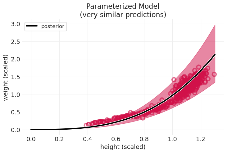
回顾:几何人#
大部分 \(H \rightarrow W\) 是由于长度和体积之间的关系
身体形状的变化解释了儿童的拟合效果不佳——这就是比例 \(p\) 随年龄变化可能有助于改进模型的地方
尽可能推迟统计思考通常会得到更好的统计模型
不思考你实际测量的内容就没有经验主义
选择、观察和学习策略 🟦🟥#
实验#
多数选择
三个不同的孩子选择 🟥 并获得奖励
少数选择
一个孩子选择 🟨 三次,并获得三个奖励
未选择
🟦 未被任何孩子选择
所选颜色的总证据是 🟥,🟥,🟥,🟨,🟨,🟨
科学思考,模拟数据#
np.random.seed(123)
N_SIMULATED_CHILDREN = 100

# half of children take the random color strategy
y_random = np.random.choice([1, 2, 3], N_SIMULATED_CHILDREN // 2, replace=True)

# the other half follow the majority -> p(majority) = 0.5
y_majority = np.random.choice([2], N_SIMULATED_CHILDREN // 2, replace=True)

perm_idx = np.random.permutation(np.arange(N_SIMULATED_CHILDREN))
y_simulated = np.concatenate([y_random, y_majority])[perm_idx]
plt.subplots(figsize=(6, 5))
counts, _ = np.histogram(y_random, bins=3)
strategy_labels = ["unchosen", "majority", "minority"]
strategy_colors = ["C1", "C0", "C3"]
for ii, (cnt, l, c) in enumerate(zip(counts, strategy_labels, strategy_colors)):
    plt.bar(ii, cnt, color=c, width=0.1, label="random choosers")
    if ii == 1:
        plt.bar(
            1,
            len(y_majority),
            bottom=cnt,
            color=c,
            width=0.1,
            label="majority followers",
            hatch="\\",
        )
plt.legend()
plt.xticks([0, 1, 2], labels=strategy_labels)
plt.ylabel("frequency")
plt.title("evidence for majority followers is exaggerated");

基于状态的模型#
多数选择并不表示多数偏好,因为有多种策略可能导致该选择
相反,从潜在策略空间中推断未观察到的策略
策略空间#
多数选择:选择多数演示者选择的颜色
少数选择:选择少数演示者选择的颜色
特立独行:选择未选择的颜色
随机颜色:随机选择一种颜色
这表示我们不知道是什么导致了颜色选择,但该策略不受演示者行为的限制
例如,可能是选择者最喜欢的颜色
跟随第一个:选择第一个孩子选择的颜色(可以想象有一个“跟随最后一个”的类似物)
首因效应
基于状态的统计模型#
def strategy_logp(y, p, majority_first):
    """
    y: observation
    p: prior
    majority_first: whether the majority choice was shown first before this decision was made
    """
    SWITCH = pm.math.switch
    EQ = pm.math.eq
    N_STRATEGIES = 5

    # reset params
    theta = [0] * N_STRATEGIES
    # p(data)
    theta[0] = SWITCH(EQ(y, 2), 1, 0)  # majority
    theta[1] = SWITCH(EQ(y, 3), 1, 0)  # minority
    theta[2] = SWITCH(EQ(y, 1), 1, 0)  # maverick
    theta[3] = pm.math.ones_like(y) * 1.0 / 3.0  # random color
    theta[4] = SWITCH(  # follow-first
        EQ(majority_first, 1), SWITCH(EQ(y, 2), 1, 0), SWITCH(EQ(y, 3), 1, 0)
    )

    # log probability -> log(p_S * P(y_i | S))
    for si in range(N_STRATEGIES):
        theta[si] = pm.math.log(p[si]) + pm.math.log(theta[si])

    return pm.math.logsumexp(theta, axis=0)


STRATEGY = ["majority", "minority", "maverick", "random color", "follow first"]


def fit_child_strategy_model(data):

    Y = data.y.values.astype(int)
    MAJORITY_FIRST = data.majority_first.values.astype(int)

    with pm.Model(coords={"strategy": STRATEGY}) as child_strategy_model:
        # Prior
        p = pm.Dirichlet("p", np.array([4, 4, 4, 4, 4]), dims="strategy")

        # Likelihood
        pm.CustomDist("Y", p, MAJORITY_FIRST, logp=strategy_logp, observed=Y)
        child_strategy_inference = pm.sample()

    return child_strategy_model, child_strategy_inference
将策略模型拟合到模拟数据#
BOXES_SIMULATED = pd.DataFrame(
    {
        "y": y_simulated,
        "majority_first": stats.bernoulli(p=0.5).rvs(
            size=N_SIMULATED_CHILDREN
        ),  # decouple first choice from strategy, "follow first" strategy should be near zero
    }
)
child_strategy_model_simulated, child_strategy_inference_simulated = fit_child_strategy_model(
    BOXES_SIMULATED[:5]
)
pm.plot_forest(child_strategy_inference_simulated, var_names=["p"], combined=True);
Initializing NUTS using jitter+adapt_diag...
Multiprocess sampling (4 chains in 4 jobs)
NUTS: [p]
Sampling 4 chains for 1_000 tune and 1_000 draw iterations (4_000 + 4_000 draws total) took 2 seconds.
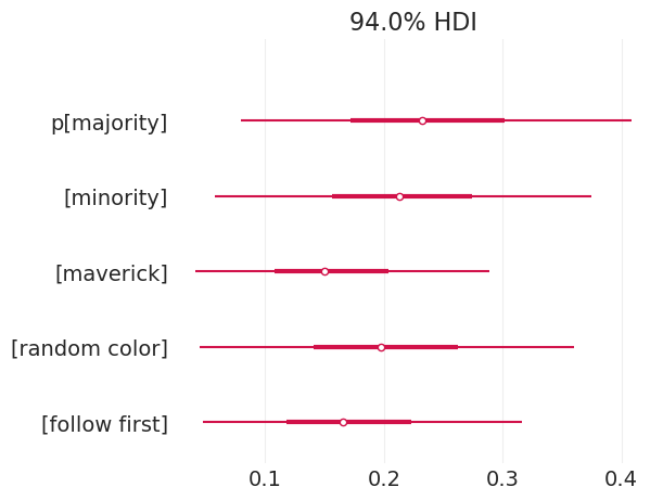
我们可以看到,我们能够恢复多数策略的模拟概率,即 0.5。
将策略模型拟合到真实数据#
BOXES = utils.load_data("Boxes")

child_strategy_model, child_strategy_inference = fit_child_strategy_model(BOXES[:5])

pm.plot_forest(child_strategy_inference, var_names=["p"], combined=True);
Initializing NUTS using jitter+adapt_diag...
Multiprocess sampling (4 chains in 4 jobs)
NUTS: [p]
Sampling 4 chains for 1_000 tune and 1_000 draw iterations (4_000 + 4_000 draws total) took 2 seconds.
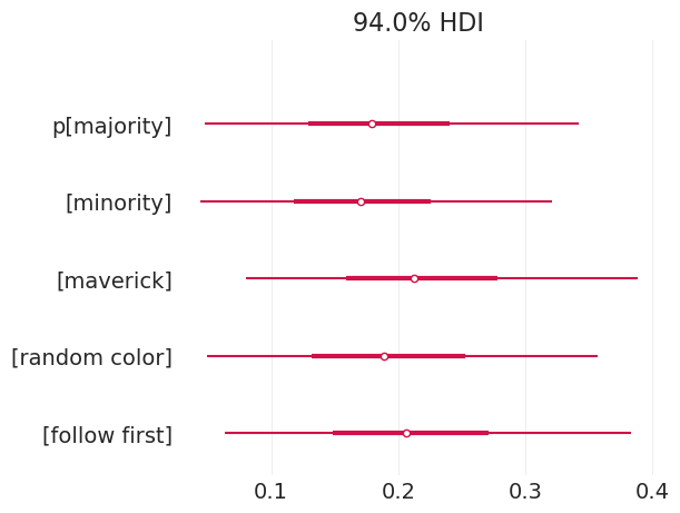
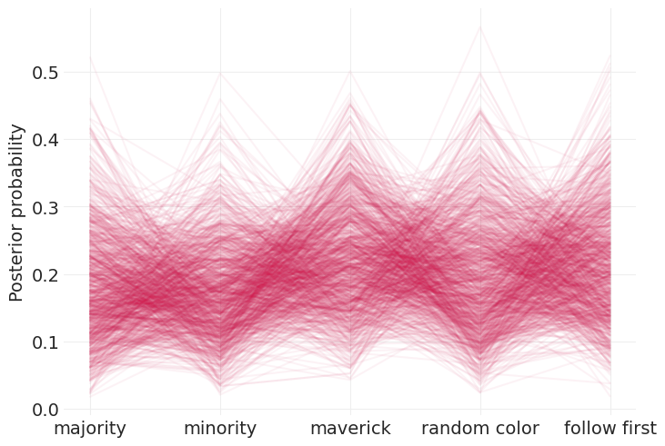
多数策略有大量的证据
跟随第一个策略有大量的证据
随机颜色具有很大的方差
困扰着实验,因为随机选择总是可以解释掉其他策略的证据
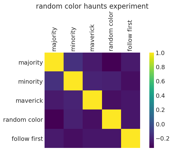
我们可以通过查看每种策略的 \(p\) 值的相关性来验证这一点:‘随机颜色’策略与所有其他策略呈负相关
posterior_ps = child_strategy_inference.posterior["p"][0, :].values.T
xs = np.arange(5)
plt.plot(xs, posterior_ps, color="C0", alpha=0.05)
plt.xticks(xs, labels=STRATEGY)
plt.ylabel("Posterior probability");
strategy_corrs = np.corrcoef(posterior_ps)

fig, ax = plt.subplots()
cax = ax.matshow(strategy_corrs)
ax.grid(None)
ax.set_xticks(np.arange(5))
ax.set_yticks(np.arange(5))
ax.set_xticklabels(STRATEGY, rotation=90)
ax.set_yticklabels(STRATEGY)
fig.colorbar(cax)
ax.set_title("random color haunts experiment");
回顾:基于状态的模型#
想要:未观察到的潜在状态(例如,策略、知识状态)
拥有:发射
仍然可以根据排放学习状态
通常有很多不确定性
替代方案是运行不正确的分析(例如,运行分类回归)
在策略中存在策略或期望结果的大量应用
运动规划
学习
家庭规划
种群动态#
潜在状态是时变的
示例:生态动态;不同物种随时间变化的数目
估计量:
不同物种如何相互作用;相互作用如何影响种群动态
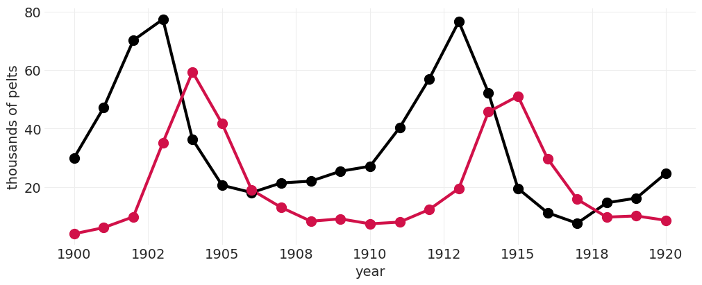
具体来说,猞猁和野兔(兔)的种群如何随时间相互作用?
POPULATION = utils.load_data("Lynx_Hare")
POPULATION
| 年份 | 猞猁 | 野兔 | |
|---|---|---|---|
| 0 | 1900 | 4.0 | 30.0 |
| 1 | 1901 | 6.1 | 47.2 |
| 2 | 1902 | 9.8 | 70.2 |
| 3 | 1903 | 35.2 | 77.4 |
| 4 | 1904 | 59.4 | 36.3 |
| 5 | 1905 | 41.7 | 20.6 |
| 6 | 1906 | 19.0 | 18.1 |
| 7 | 1907 | 13.0 | 21.4 |
| 8 | 1908 | 8.3 | 22.0 |
| 9 | 1909 | 9.1 | 25.4 |
| 10 | 1910 | 7.4 | 27.1 |
| 11 | 1911 | 8.0 | 40.3 |
| 12 | 1912 | 12.3 | 57.0 |
| 13 | 1913 | 19.5 | 76.6 |
| 14 | 1914 | 45.7 | 52.3 |
| 15 | 1915 | 51.1 | 19.5 |
| 16 | 1916 | 29.7 | 11.2 |
| 17 | 1917 | 15.8 | 7.6 |
| 18 | 1918 | 9.7 | 14.6 |
| 19 | 1919 | 10.1 | 16.2 |
| 20 | 1920 | 8.6 | 24.7 |
from matplotlib import ticker


def plot_population(data, ax=None):

    if ax is None:
        _, ax = plt.subplots(figsize=(10, 4))

    plt.scatter(data.Year, data.Hare, color="k", label="Lepus", zorder=100, s=100)
    utils.plot_line(data.Year, data.Hare, color="k", label="Lepus")

    plt.scatter(data.Year, data.Lynx, color="C0", label="Lynx", zorder=100, s=100)
    utils.plot_line(data.Year, data.Lynx, color="C0", label="Lynx")

    plt.gca().xaxis.set_major_formatter(ticker.FormatStrFormatter("%.0f"))
    plt.xlabel("year")
    plt.ylabel("thousands of pelts")


plot_population(POPULATION)
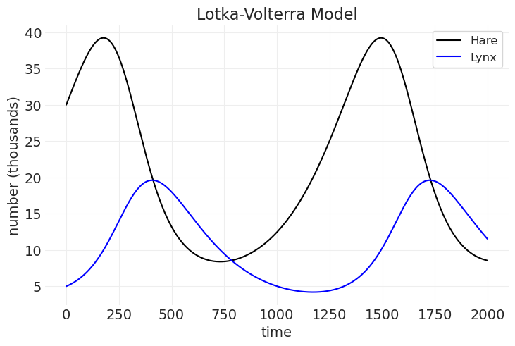
Lotka-Volterra 模型#
野兔种群模型 🐰#
猞猁种群模型 😸#
from numba import njit
from scipy.integrate import odeint


@njit
def lotka_volterra_diffeq(X, t, theta):
    # Unpack
    H, L = X
    bH, mH, bL, mL, _, _ = theta

    # Diff equations
    dH_dt = H * (bH - mH * L)
    dL_dt = L * (bL * H - mL)
    return [dH_dt, dL_dt]


def simulate_population_dynamics(
    initial_hares=30,
    initial_lynxes=5,
    birth_rate_hare=0.5,
    mortatily_rate_hare=0.05,
    birth_rate_lynx=0.025,
    mortality_rate_lynx=0.5,
    n_time_points=20,
    dt=1,
):
    time = np.arange(0, n_time_points, dt)
    theta = np.array(
        [
            birth_rate_hare,
            mortatily_rate_hare,
            birth_rate_lynx,
            mortality_rate_lynx,
            initial_hares,
            initial_lynxes,
        ]
    )
    HL = odeint(func=lotka_volterra_diffeq, y0=theta[-2:], t=time, args=(theta,))
    return HL[:, 0], HL[:, 1]


# Simulation with parameters shown in Figure 16.7 of the book (2nd edition)
hare_population, lynx_population = simulate_population_dynamics(
    initial_hares=30,
    initial_lynxes=5,
    birth_rate_hare=0.5,
    mortatily_rate_hare=0.05,
    birth_rate_lynx=0.025,
    mortality_rate_lynx=0.5,
    n_time_points=20,
    dt=0.01,
)
plt.plot(hare_population, color="k", label="Hare")
plt.plot(lynx_population, color="blue", label="Lynx")
plt.xlabel("time")
plt.ylabel("number (thousands)")
plt.legend()
plt.title("Lotka-Volterra Model");
统计模型#
先验预测模拟#
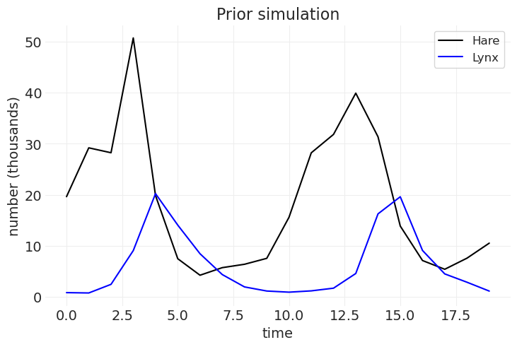
def sample_prior(random_seed=None):
    if random_seed is not None:
        np.random.seed(random_seed)

    # Initial population
    population_prior = stats.lognorm(np.log(10), 1)
    initial_hares_population = population_prior.rvs()
    initial_lynx_population = population_prior.rvs()

    # Observation model, probability of getting trapped
    trapped_prior = stats.beta(40, 200)
    p_trapped_hare = trapped_prior.rvs()
    p_trapped_lynx = trapped_prior.rvs()

    initial_hares = initial_hares_population * p_trapped_hare
    initial_lynxes = initial_lynx_population * p_trapped_lynx

    # Birth/mortality rates
    birth_rate_hare = stats.halfnorm(0.5, 0.5).rvs()
    birth_rate_lynx = stats.halfnorm(0.05, 0.05).rvs()

    mortality_rate_hare = stats.halfnorm(0.05, 0.05).rvs()
    mortality_rate_lynx = stats.halfnorm(0.5, 0.5).rvs()

    hare_population, lynx_population = simulate_population_dynamics(
        initial_hares,
        initial_lynxes,
        birth_rate_hare,
        mortality_rate_hare,
        birth_rate_lynx,
        mortality_rate_lynx,
        n_time_points=20,
        dt=1,
    )

    # Multiplicative noise
    hare_population *= 1 + np.random.rand(len(hare_population))
    lynx_population *= 1 + np.random.rand(len(lynx_population))

    plt.plot(hare_population, color="k", label="Hare")
    plt.plot(lynx_population, color="blue", label="Lynx")
    plt.xlabel("time")
    plt.ylabel("number (thousands)")
    plt.title("Prior simulation")
    plt.legend()

    return {
        "initial_hares_population": initial_hares_population,
        "initial_lynx_population": initial_lynx_population,
        "p_trapped_hare": p_trapped_hare,
        "p_trapped_lynx": p_trapped_lynx,
        "initial_hares": initial_hares,
        "initial_lynxes": initial_lynxes,
        "birth_rate_hare": birth_rate_hare,
        "mortality_rate_hare": mortality_rate_hare,
        "birth_rate_lynx": birth_rate_lynx,
        "mortality_rate_lynx": mortality_rate_lynx,
        "hare_population": hare_population,
        "lynx_population": lynx_population,
    }


prior_samples = sample_prior(random_seed=3)
SIMULATED_POPULATION = pd.DataFrame(
    {
        "Year": np.arange(1900, 1900 + len(prior_samples["hare_population"])),
        "Hare": prior_samples["hare_population"],
        "Lynx": prior_samples["lynx_population"],
    }
)
prior_samples
{'initial_hares_population': 62.46508314413322,
 'initial_lynx_population': 3.73218341358194,
 'p_trapped_hare': 0.18755284355997892,
 'p_trapped_lynx': 0.16310620806753454,
 'initial_hares': 11.715503966892694,
 'initial_lynxes': 0.6087422844018971,
 'birth_rate_hare': 0.5219090844879641,
 'mortality_rate_hare': 0.11569323766813411,
 'birth_rate_lynx': 0.07386090151797514,
 'mortality_rate_lynx': 0.9423111902497923,
 'hare_population': array([19.63817095, 29.19826078, 28.23651683, 50.71810838, 19.84793473,
         7.47923655,  4.24935002,  5.73155482,  6.39410051,  7.5552296 ,
        15.60151539, 28.22202333, 31.82844508, 39.9041958 , 31.36096064,
        13.88083494,  7.12609809,  5.41608361,  7.59162182, 10.5313164 ]),
 'lynx_population': array([ 0.83884324,  0.77317152,  2.46052459,  9.07240807, 20.22343338,
        14.06319061,  8.45831069,  4.3774741 ,  1.95684229,  1.155288  ,
         0.928704  ,  1.18563233,  1.71134393,  4.58554862, 16.26497351,
        19.61763805,  9.09467367,  4.50667308,  2.87452939,  1.14325939])}
实施统计模型#
PyMC 实施细节#
PyMC 有一个内置的 ODE 求解器,但该求解器的文档警告说它非常慢,并建议我们使用 Sunode ODE Solver。据我所知,目前 sunode 求解器不适用于 Mac M1(即,它在 conda-forge 上不可用,并且从源代码安装在 ARM64 芯片组上有点混乱)。
实际上,我发现 PyMC 中的内置 ODE 求解器 (pm.ode.DifferentialEquation) 对于构建和调试模型来说是令人望而却步的(每个模型的采样时间超过一小时;在这种速度下迭代非常困难)。作为一种替代方法,我正在使用 PyMC 文档中 Lotke-Volterra 示例中概述的实现。该方法是使用 Pytensor 的 as_op 装饰器包装 scipy 的 odeint 函数,以便可以通过 PyMC 使用可变输入/输出类型。这允许我们使用非基于梯度的采样器(例如 Slice 采样器),这些采样器对于嵌入 ODE 集成的奇异模型更加宽容。
⚠️ 这些模型对起始条件非常敏感,并且我无法使用讲座中建议的先验使模型收敛。相反,我们对数据执行初始最小二乘拟合,并使用得到的最小二乘参数估计来告知我们的先验。
# Plotting helpers


def plot_data(data):
    utils.plot_scatter(data.Year, data.Hare, color="k", zorder=100, alpha=1)
    utils.plot_scatter(data.Year, data.Lynx, color="blue", zorder=100, alpha=1)


def plot_model_trace(inference_df, row_idx, lw=1, alpha=0.2, label=False):

    cols = ["bH", "mH", "bL", "mL", "initial_H", "initial_L"]
    theta = inference_df.loc[row_idx, cols].values
    p_trapped = inference_df.loc[row_idx, ["p_trapped_H", "p_trapped_L"]].values

    time = np.arange(1900, 1921, 0.01)

    # Run dynamics with model params
    HL = odeint(func=lotka_volterra_diffeq, y0=theta[-2:], t=time, args=(theta,))

    label_H = "Hare" if label else None
    label_L = "Lynx" if label else None
    hare_pelts = HL[:, 0] * p_trapped[0]
    lynx_pelts = HL[:, 1] * p_trapped[1]
    utils.plot_line(xs=time, ys=hare_pelts, color="k", alpha=0.1, label=label_H)
    utils.plot_line(xs=time, ys=lynx_pelts, color="blue", alpha=0.1, label=label_L)


def plot_population_model_posterior(
    inference,
    n_samples=25,
    title=None,
    plot_model_kwargs=dict(lw=1, alpha=0.2),
):
    inference_df = inference.posterior.sel(chain=0).to_dataframe()

    for row_idx in range(n_samples):
        label = row_idx == 0
        plot_model_trace(inference_df, row_idx, label=label)

    plt.legend()
    plt.title(title, fontsize=16)
import pytensor.tensor as pt

from pytensor.compile.ops import as_op
from scipy.optimize import least_squares


def fit_lotka_volterra_model(data, theta_0=None):
    # Data
    H = data.Hare.values.astype(float)
    L = data.Lynx.values.astype(float)
    TIMES = data.Year.astype(float)

    # Step 0, get informed priors using Least Squares
    def ode_model_residuals(theta):
        # Calculates residuals for Lotka-Volterra model, based on a given state of params
        return (
            data[["Hare", "Lynx"]]
            - odeint(func=lotka_volterra_diffeq, y0=theta[-2:], t=data.Year, args=(theta,))
        ).values.flatten()

    # Least squares solution using the scipy's solver
    theta_0 = np.array([0.5, 0.025, 0.025, 0.75, H[0], L[0]]) if theta_0 is None else theta_0
    lstsq_solution = least_squares(ode_model_residuals, x0=theta_0)

    # Pack solution into a dictionary for more-readable code
    lstsq = {}
    parameter_names = ["bH", "mH", "bL", "mL", "H0", "L0"]
    for k, v in zip(parameter_names, lstsq_solution.x):
        lstsq[k] = v
    print("Initial Least Square Param Estimates:\n", lstsq)

    # Decorate so that input and output have Pytensor types.
    # This allows `odeint` to be available to PyMC as a valid operation
    @as_op(itypes=[pt.dvector], otypes=[pt.dmatrix])
    def pytensor_lotka_volterra_diffeq(theta):
        return odeint(func=lotka_volterra_diffeq, y0=theta[-2:], t=TIMES, args=(theta,))

    with pm.Model() as model:

        # Initial population priors
        initial_H = pm.LogNormal("initial_H", np.log(10), 1, initval=lstsq["H0"])
        initial_L = pm.LogNormal("initial_L", np.log(10), 1, initval=lstsq["L0"])

        # Hare param priors
        bH = pm.TruncatedNormal("bH", mu=lstsq["bH"], sigma=0.1, lower=0.0, initval=lstsq["bH"])
        mH = pm.TruncatedNormal("mH", mu=lstsq["mH"], sigma=0.05, lower=0.0, initval=lstsq["mH"])

        # Lynx param priors
        bL = pm.TruncatedNormal("bL", mu=lstsq["bL"], sigma=0.05, lower=0.0, initval=lstsq["bL"])
        mL = pm.TruncatedNormal("mL", mu=lstsq["mL"], sigma=0.1, lower=0.0, initval=lstsq["mL"])

        # Run dynamical system with current params/initial pops
        ode_solution = pytensor_lotka_volterra_diffeq(
            pm.math.stack([bH, mH, bL, mL, initial_H, initial_L])
        )

        # Observation model, probability of being trapped
        p_trapped_H = pm.Beta("p_trapped_H", 40, 200)
        p_trapped_L = pm.Beta("p_trapped_L", 40, 200)

        # Measurement error variance
        sigma_H = pm.Exponential("sigma_H", 1)
        sigma_L = pm.Exponential("sigma_L", 1)

        # Hare likelihood
        population_H = ode_solution[:, 0]
        mu_H = pm.math.log(population_H * p_trapped_H)
        pm.LogNormal("H", mu=mu_H, sigma=sigma_H, observed=H)

        # Lynx likelihood
        population_L = ode_solution[:, 1]
        mu_L = pm.math.log(population_L * p_trapped_L)
        pm.LogNormal("L", mu=mu_L, sigma=sigma_L, observed=L)

        inference = pm.sample()

    return model, inference
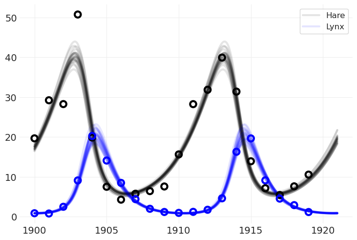
将模型拟合到模拟数据#
lv_model_simualted, lt_inference_simulated = fit_lotka_volterra_model(
    SIMULATED_POPULATION,
    theta_0=np.array(
        [
            prior_samples["birth_rate_hare"],
            prior_samples["mortality_rate_hare"],
            prior_samples["birth_rate_lynx"],
            prior_samples["mortality_rate_lynx"],
            prior_samples["initial_hares"],
            prior_samples["initial_lynxes"],
        ]
    ),
)
Initial Least Square Param Estimates:
 {'bH': 0.4206452785407346, 'mH': 0.07341907569799343, 'bL': 0.06444364541512093, 'mL': 1.1815068440602556, 'H0': 17.997517919089947, 'L0': 0.575807704356167}
Multiprocess sampling (4 chains in 4 jobs)
CompoundStep
>CompoundStep
>>Slice: [initial_H]
>>Slice: [initial_L]
>>Slice: [bH]
>>Slice: [mH]
>>Slice: [bL]
>>Slice: [mL]
>NUTS: [p_trapped_H, p_trapped_L, sigma_H, sigma_L]
Sampling 4 chains for 1_000 tune and 1_000 draw iterations (4_000 + 4_000 draws total) took 37 seconds.
There were 2 divergences after tuning. Increase `target_accept` or reparameterize.
The rhat statistic is larger than 1.01 for some parameters. This indicates problems during sampling. See https://arxiv.org/abs/1903.08008 for details
The effective sample size per chain is smaller than 100 for some parameters.  A higher number is needed for reliable rhat and ess computation. See https://arxiv.org/abs/1903.08008 for details
plot_population_model_posterior(lt_inference_simulated)
plot_data(SIMULATED_POPULATION)
将模型拟合到真实数据#
lv_model, lt_inference = fit_lotka_volterra_model(POPULATION)
Initial Least Square Param Estimates:
 {'bH': 0.4812006467847881, 'mH': 0.024831840848356775, 'bL': 0.02753293803703795, 'mL': 0.926016346040929, 'H0': 34.914136989883445, 'L0': 3.8618647177263425}
Multiprocess sampling (4 chains in 4 jobs)
CompoundStep
>CompoundStep
>>Slice: [initial_H]
>>Slice: [initial_L]
>>Slice: [bH]
>>Slice: [mH]
>>Slice: [bL]
>>Slice: [mL]
>NUTS: [p_trapped_H, p_trapped_L, sigma_H, sigma_L]
Sampling 4 chains for 1_000 tune and 1_000 draw iterations (4_000 + 4_000 draws total) took 36 seconds.
The rhat statistic is larger than 1.01 for some parameters. This indicates problems during sampling. See https://arxiv.org/abs/1903.08008 for details
The effective sample size per chain is smaller than 100 for some parameters.  A higher number is needed for reliable rhat and ess computation. See https://arxiv.org/abs/1903.08008 for details
绘制后验#
请注意,我们绘制的后验网格比数据本身更精细。这可以使用后验参数来完成,并以比数据更高的分辨率运行 ODE
plot_population_model_posterior(lt_inference)
plot_data(POPULATION)
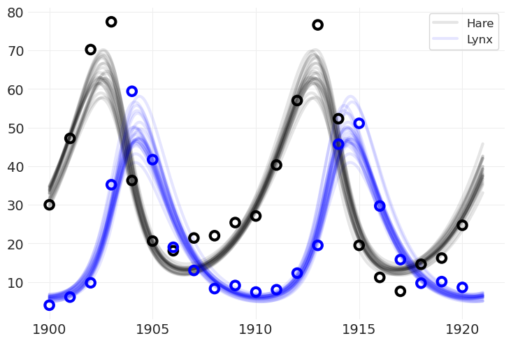
回顾:种群动态#
生态系统比这个简单的模型复杂得多
例如,许多其他动物捕食野兔
没有因果结构/模型;理解政策干预几乎没有希望
许可声明#
此示例库中的所有笔记本均根据 MIT 许可证 提供,该许可证允许修改和再分发以用于任何用途,前提是保留版权和许可声明。
引用 PyMC 示例#
要引用此笔记本,请使用 Zenodo 为 pymc-examples 存储库提供的 DOI。
重要
许多笔记本改编自其他来源:博客、书籍…… 在这种情况下,您也应该引用原始来源。
还请记住引用您的代码使用的相关库。
这是一个 bibtex 格式的引用模板
@incollection{citekey,
  author    = "<notebook authors, see above>",
  title     = "<notebook title>",
  editor    = "PyMC Team",
  booktitle = "PyMC examples",
  doi       = "10.5281/zenodo.5654871"
}
渲染后可能看起来像
社会顺应性#
在目睹上述数据后,其他孩子在选择颜色时采取什么策略?
孩子们是否复制 多数选择 ——即多数人的 策略?
问题:无法直接观察策略,只能观察选择
多数选择与许多策略一致
随机选择颜色 \(\rightarrow 1/3\)
随机演示者 \(\rightarrow 3/4\)
随机演示 \(\rightarrow 1/2\)