贝叶斯参数生存分析

import warnings

import arviz as az
import numpy as np
import pymc as pm
import pytensor.tensor as pt
import scipy as sp
import seaborn as sns

from matplotlib import pyplot as plt
from matplotlib.ticker import StrMethodFormatter
from statsmodels import datasets

print(f"Running on PyMC v{pm.__version__}")

Running on PyMC v5.16.2

%config InlineBackend.figure_format = 'retina'
az.style.use("arviz-darkgrid")
warnings.filterwarnings("ignore")

生存分析 研究的是从受试者开始接受观察到受试者经历感兴趣事件之间的时间分布。生存分析的基本挑战之一（也使其在数学上很有趣）是，一般来说，并非每个受试者都会在我们进行分析之前经历感兴趣的事件。更具体地说，如果我们正在研究癌症治疗到死亡之间的时间（正如我们将在本文中做的那样），我们通常希望在每个受试者死亡之前分析我们的数据。这种现象称为截尾，是生存分析的基础。

这篇文章说明了在 PyMC 中进行贝叶斯生存分析的参数方法。参数生存模型比半参数模型更易于实施和理解；在统计学上，当正确指定时，它们也比非参数或半参数方法更有效。有关半参数 Cox 比例风险模型的示例，您可以阅读这篇博文，但请注意，该博文使用了旧版本的 PyMC，并且在 PyMC 中实施半参数模型涉及一些相当复杂的 numpy 代码和不明显的概率论等价性。

我们将分析来自 R 的 HSAUR 包的 乳房切除术数据。

sns.set()
blue, green, red, purple, gold, teal = sns.color_palette(n_colors=6)

pct_formatter = StrMethodFormatter("{x:.1%}")

df = datasets.get_rdataset("mastectomy", "HSAUR", cache=True).data.assign(
    metastized=lambda df: 1.0 * (df.metastized == "yes"), event=lambda df: 1.0 * df.event
)
df.head()

	时间	事件	转移
0	23	1.0	0.0
1	47	1.0	0.0
2	69	1.0	0.0
3	70	0.0	0.0
4	100	0.0	0.0

time 列表示乳腺癌患者乳房切除术后的生存时间，以月为单位。 event 列指示观察是否被截尾。如果 event 为 1，则在研究期间观察到患者死亡；如果 event 为零，则患者在研究结束时仍然存活，并且他们的生存时间被截尾。 metastized 列指示癌症是否在乳房切除术前已转移。在这篇文章中，我们将使用贝叶斯参数生存回归来量化癌症转移和未转移患者的生存时间差异。

加速失效时间模型

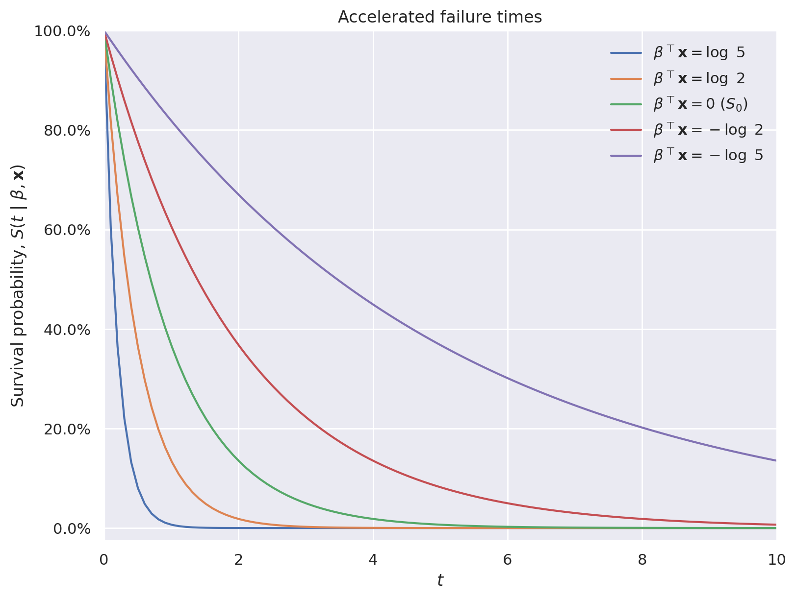
加速失效时间模型 是最常见的参数生存回归模型类型。生存分析的基本量是生存函数；如果 \(T\) 是表示事件发生时间的随机变量，则生存函数为 \(S(t) = P(T > t)\)。加速失效时间模型将协变量 \(\mathbf{x}\) 纳入生存函数，如下所示：

\[S(t\ |\ \beta, \mathbf{x}) = S_0\left(\exp\left(\beta^{\top} \mathbf{x}\right) \cdot t\right),\]

其中 \(S_0(t)\) 是固定的基线生存函数。这些模型被称为“加速失效时间”，因为当 \(\beta^{\top} \mathbf{x} > 0\) 时，\(\exp\left(\beta^{\top} \mathbf{x}\right) \cdot t > t\)，因此协变量的作用是加速所讨论个体有效的时间流逝。下图使用指数生存函数说明了这种现象。

S0 = sp.stats.expon.sf

fig, ax = plt.subplots(figsize=(8, 6))

t = np.linspace(0, 10, 100)

ax.plot(t, S0(5 * t), label=r"$\beta^{\top} \mathbf{x} = \log\ 5$")
ax.plot(t, S0(2 * t), label=r"$\beta^{\top} \mathbf{x} = \log\ 2$")
ax.plot(t, S0(t), label=r"$\beta^{\top} \mathbf{x} = 0$ ($S_0$)")
ax.plot(t, S0(0.5 * t), label=r"$\beta^{\top} \mathbf{x} = -\log\ 2$")
ax.plot(t, S0(0.2 * t), label=r"$\beta^{\top} \mathbf{x} = -\log\ 5$")

ax.set_xlim(0, 10)
ax.set_xlabel(r"$t$")

ax.yaxis.set_major_formatter(pct_formatter)
ax.set_ylim(-0.025, 1)
ax.set_ylabel(r"Survival probability, $S(t\ |\ \beta, \mathbf{x})$")

ax.legend(loc=1)
ax.set_title("Accelerated failure times");

加速失效时间模型等效于 \(T\) 的对数线性模型：

\[Y = \log T = \beta^{\top} \mathbf{x} + \varepsilon.\]

误差项 \(\varepsilon\) 的分布选择决定了加速失效时间模型的基线生存函数 \(S_0\)。下表显示了 \(\varepsilon\) 的分布与几种常见加速失效时间模型的 \(S_0\) 之间的对应关系。

对数线性误差分布 (\(\varepsilon\))	基线生存函数 (\(S_0\))
正态	对数正态
极值 (耿贝尔)	威布尔
逻辑斯蒂	对数逻辑斯蒂

加速失效时间模型通常以其基线生存函数 \(S_0\) 命名。这篇文章的其余部分将展示如何在 PyMC 中使用乳房切除术数据实现威布尔和对数逻辑斯蒂生存回归模型。

威布尔生存回归

在本例中，协变量为 \(\mathbf{x}_i = \left(1\ x^{\textrm{met}}_i\right)^{\top}\)，其中

\[\begin{split} \begin{align*} x^{\textrm{met}}_i & = \begin{cases} 0 & \textrm{如果第 } i\textrm{-位患者的癌症未转移} \\ 1 & \textrm{如果第 } i\textrm{-位患者的癌症已转移} \end{cases}. \end{align*} \end{split}\]

我们构建协变量矩阵 \(\mathbf{X}\)。

n_patient, _ = df.shape

X = np.empty((n_patient, 2))
X[:, 0] = 1.0
X[:, 1] = df.metastized

with pm.Model() as weibull_model:
    predictors = pm.Data("predictors", X)

数据的似然性分为两部分指定，一部分用于未截尾样本，一部分用于截尾样本。由于 \(Y = \eta + \varepsilon\)，并且 \(\varepsilon \sim \textrm{Gumbel}(0, s)\)，\(Y \sim \textrm{Gumbel}(\eta, s)\)。对于未截尾的生存时间，似然性实现为

with weibull_model:
    censored = pm.Data("censored", df.event.values == 0.0)

我们将观察到的时间转换为对数尺度并进行标准化。

y = np.log(df.time.values)
y_std = (y - y.mean()) / y.std()

with weibull_model:
    y_obs = pm.Data("y_obs", y_std[df.event.values == 1.0])
    y_cens = pm.Data("y_cens", y_std[df.event.values == 0.0])

我们在回归系数上放置独立的、模糊的正态先验分布：

\[\beta \sim N(0, 5^2 I_2).\]

with weibull_model:
    beta = pm.Normal("beta", mu=0.0, sigma=5.0, shape=2)

协变量 \(\mathbf{x}\) 通过 \(\eta = \beta^{\top} \mathbf{x}\) 影响 \(Y = \log T\) 的值。

with weibull_model:
    eta = beta.dot(predictors.T)

对于威布尔回归，我们使用

\[\begin{split} \begin{align*} \varepsilon & \sim \textrm{Gumbel}(0, s) \\ s & \sim \textrm{HalfNormal(5)}. \end{align*} \end{split}\]

with weibull_model:
    s = pm.HalfNormal("s", 5.0)

with weibull_model:
    events = pm.Gumbel("events", eta[~censored], s, observed=y_obs)

对于截尾观察，我们只知道它们的真实生存时间超过了它们被观察的总时间。此概率由耿贝尔分布的生存函数给出：

\[P(Y \geq y) = 1 - \exp\left(-\exp\left(-\frac{y - \mu}{s}\right)\right).\]

此生存函数在下面实现。

def gumbel_sf(y, mu, sigma):
    return 1.0 - pt.exp(-pt.exp(-(y - mu) / sigma))

我们现在指定截尾观察的似然性。

with weibull_model:
    censored_like = pm.Potential("censored_like", gumbel_sf(y_cens, eta[censored], s))

我们现在从模型中采样。

SEED = 845199  # from random.org, for reproducibility

SAMPLE_KWARGS = {"chains": 4, "tune": 1000, "random_seed": [SEED + i for i in range(4)]}

with weibull_model:
    weibull_trace = pm.sample(**SAMPLE_KWARGS)

Auto-assigning NUTS sampler...
Initializing NUTS using jitter+adapt_diag...
Multiprocess sampling (4 chains in 4 jobs)
NUTS: [beta, s]

Sampling 4 chains for 1_000 tune and 1_000 draw iterations (4_000 + 4_000 draws total) took 1 seconds.

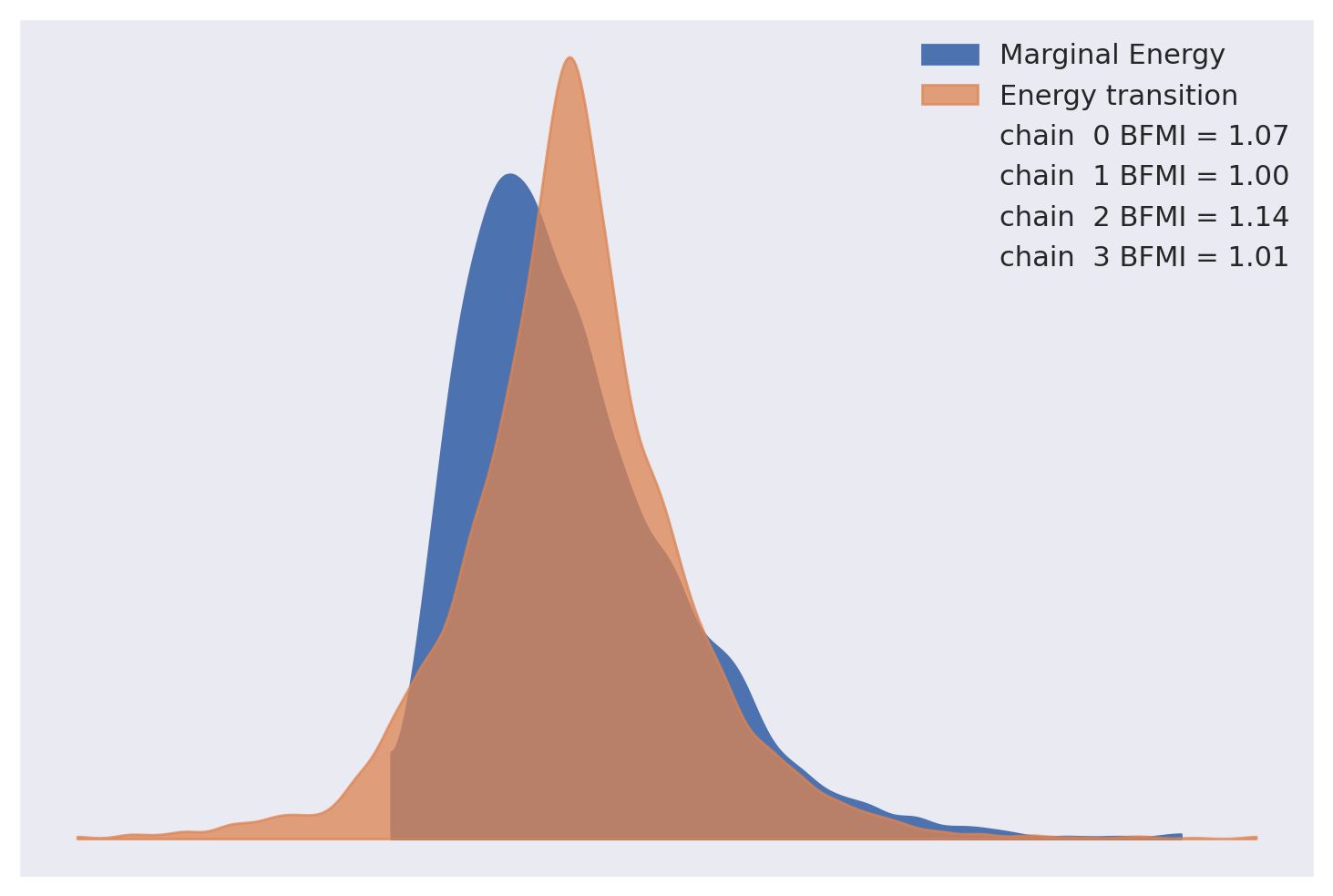
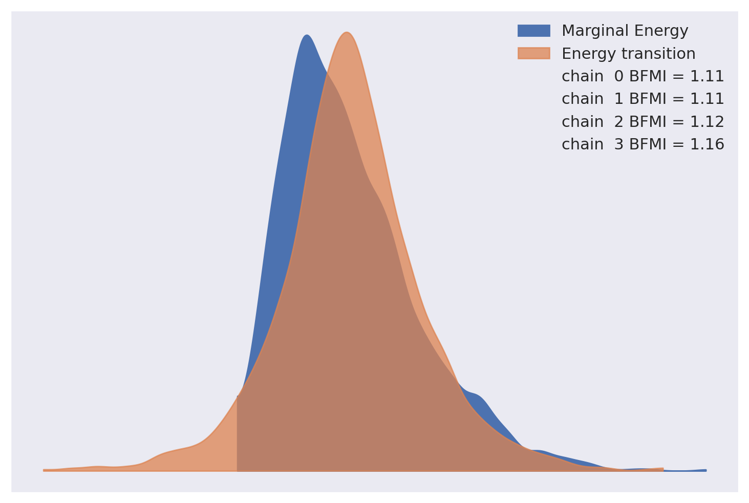
能量图和贝叶斯缺失信息分数没有引起对 NUTS 中混合不良的担忧。

az.plot_energy(weibull_trace, fill_color=("C0", "C1"));

\(\hat{R}\) 统计量也表明收敛。

max(np.max(gr_stats) for gr_stats in az.rhat(weibull_trace).values())

<xarray.DataArray 'beta' ()> Size: 8B
array(1.00442271)

xarray.DataArray

'beta'

• 1.004

  array(1.00442271)

• 坐标: (0)
• 索引: (0)
• 属性: (0)

下面我们绘制参数的后验分布。

az.plot_forest(weibull_trace, figsize=(10, 4));

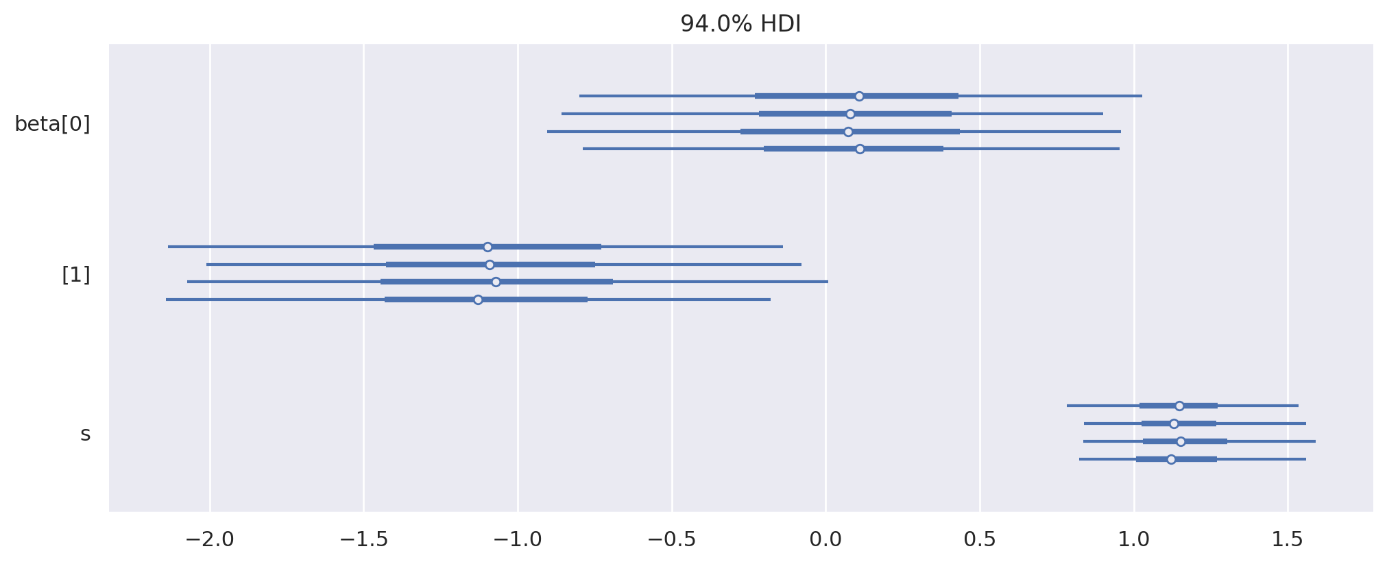
这些有些有趣（特别是 \(\beta_1\) 的后验分布与零相当好地分离），但后验预测生存曲线将更易于解释。

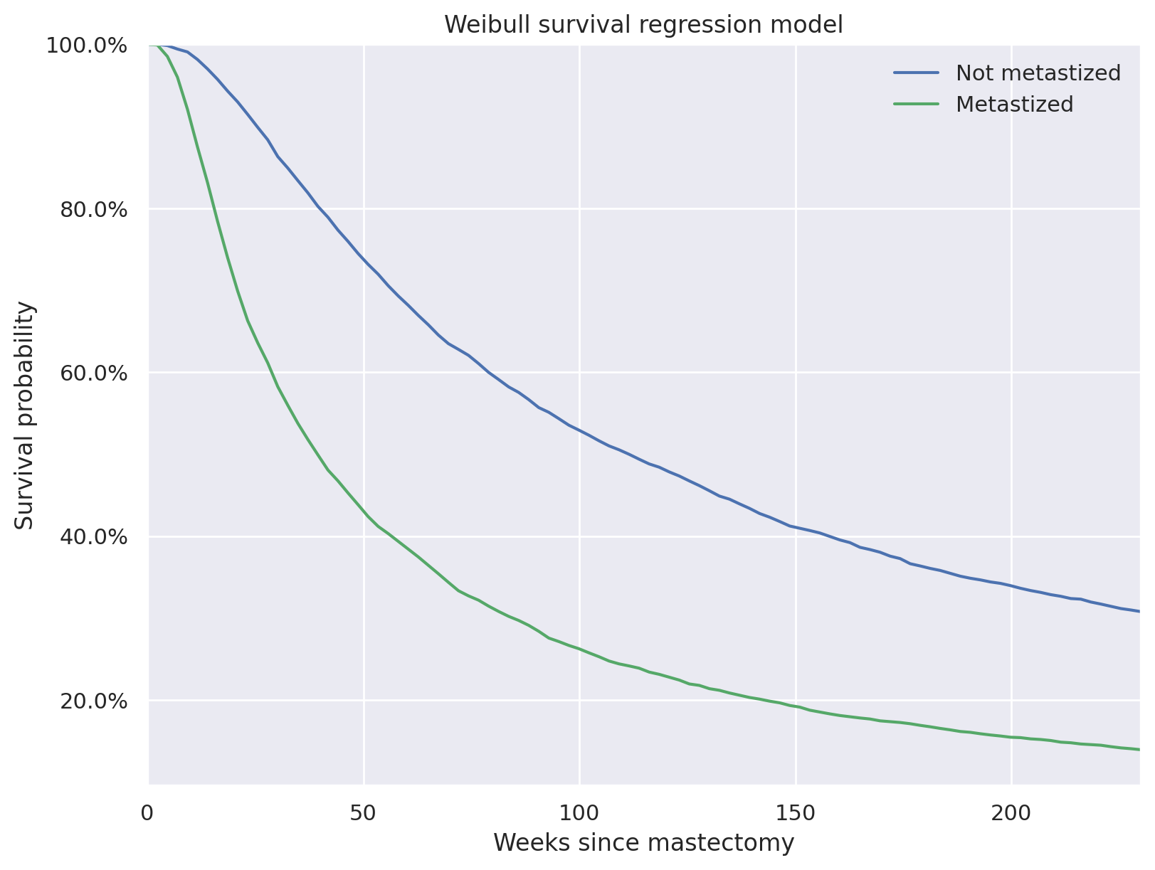
使用 Data 变量的优势在于我们现在可以更改其值以执行后验预测抽样。对于后验预测，我们将 \(X\) 设置为具有两行，一行用于癌症未转移的受试者，另一行用于癌症已转移的受试者。由于我们想要预测实际生存时间，因此后验预测行均未被截尾。

X_pp = np.empty((2, 2))
X_pp[:, 0] = 1.0
X_pp[:, 1] = [0, 1]

cens_pp = np.repeat(False, 2)

with weibull_model:
    pm.set_data(
        {"predictors": X_pp, "censored": cens_pp, "y_obs": np.zeros(2), "y_cens": np.zeros(0)}
    )

with weibull_model:
    pp_weibull_trace = pm.sample_posterior_predictive(weibull_trace)

Sampling: [events]

后验预测生存时间表明，平均而言，癌症未转移的患者比癌症已转移的患者生存时间更长。

t_plot = np.linspace(0, 230, 100)

weibull_pp_surv = np.greater_equal.outer(
    np.exp(
        y.mean()
        + y.std() * az.extract(pp_weibull_trace.posterior_predictive["events"])["events"].values
    ),
    t_plot,
)
weibull_pp_surv_mean = weibull_pp_surv.mean(axis=1)

fig, ax = plt.subplots(figsize=(8, 6))


ax.plot(t_plot, weibull_pp_surv_mean[0], c=blue, label="Not metastized")
ax.plot(t_plot, weibull_pp_surv_mean[1], c=red, label="Metastized")

ax.set_xlim(0, 230)
ax.set_xlabel("Weeks since mastectomy")

ax.set_ylim(top=1)
ax.yaxis.set_major_formatter(pct_formatter)
ax.set_ylabel("Survival probability")

ax.legend(loc=1)
ax.set_title("Weibull survival regression model");

对数逻辑斯蒂生存回归

可以通过更改 \(\varepsilon\) 的先验分布，以模块化方式指定其他加速失效时间模型。对数逻辑斯蒂模型对应于 \(\varepsilon\) 上的逻辑斯蒂先验。大多数模型规范与上面的威布尔模型相同。

with pm.Model() as log_logistic_model:
    predictors = pm.Data("predictors", X)
    censored = pm.Data("censored", df.event.values == 0.0)
    y_obs = pm.Data("y_obs", y_std[df.event.values == 1.0])
    y_cens = pm.Data("y_cens", y_std[df.event.values == 0.0])

    beta = pm.Normal("beta", 0.0, 5.0, shape=2)
    eta = beta.dot(predictors.T)

    s = pm.HalfNormal("s", 5.0)

我们使用先验 \(\varepsilon \sim \textrm{Logistic}(0, s)\)。逻辑斯蒂分布的生存函数为

\[P(Y \geq y) = 1 - \frac{1}{1 + \exp\left(-\left(\frac{y - \mu}{s}\right)\right)},\]

因此我们得到似然性

def logistic_sf(y, mu, s):
    return 1.0 - pm.math.sigmoid((y - mu) / s)

with log_logistic_model:
    events = pm.Logistic("events", eta[~censored], s, observed=y_obs)
    censored_like = pm.Potential("censored_like", logistic_sf(y_cens, eta[censored], s))

我们现在从对数逻辑斯蒂模型中采样。

with log_logistic_model:
    log_logistic_trace = pm.sample(**SAMPLE_KWARGS)

Auto-assigning NUTS sampler...
Initializing NUTS using jitter+adapt_diag...
Multiprocess sampling (4 chains in 4 jobs)
NUTS: [beta, s]

Sampling 4 chains for 1_000 tune and 1_000 draw iterations (4_000 + 4_000 draws total) took 2 seconds.

所有抽样诊断结果对于此模型看起来都不错。

az.plot_energy(log_logistic_trace, fill_color=("C0", "C1"));

max(np.max(gr_stats) for gr_stats in az.rhat(log_logistic_trace).values())

<xarray.DataArray 'beta' ()> Size: 8B
array(1.00301488)

xarray.DataArray

'beta'

• 1.003

  array(1.00301488)

• 坐标: (0)
• 索引: (0)
• 属性: (0)

同样，我们计算此模型的后验预期生存函数。

with log_logistic_model:
    pm.set_data(
        {"predictors": X_pp, "censored": cens_pp, "y_obs": np.zeros(2), "y_cens": np.zeros(0)}
    )
    pp_log_logistic_trace = pm.sample_posterior_predictive(log_logistic_trace)

Sampling: [events]

log_logistic_pp_surv = np.greater_equal.outer(
    np.exp(
        y.mean()
        + y.std()
        * az.extract(pp_log_logistic_trace.posterior_predictive["events"])["events"].values
    ),
    t_plot,
)
log_logistic_pp_surv_mean = log_logistic_pp_surv.mean(axis=1)

fig, ax = plt.subplots(figsize=(8, 6))

ax.plot(t_plot, weibull_pp_surv_mean[0], c=blue, label="Weibull, not metastized")
ax.plot(t_plot, weibull_pp_surv_mean[1], c=red, label="Weibull, metastized")

ax.plot(t_plot, log_logistic_pp_surv_mean[0], "--", c=blue, label="Log-logistic, not metastized")
ax.plot(t_plot, log_logistic_pp_surv_mean[1], "--", c=red, label="Log-logistic, metastized")

ax.set_xlim(0, 230)
ax.set_xlabel("Weeks since mastectomy")

ax.set_ylim(top=1)
ax.yaxis.set_major_formatter(pct_formatter)
ax.set_ylabel("Survival probability")

ax.legend(loc=1)
ax.set_title("Weibull and log-logistic\nsurvival regression models");

这篇文章简要介绍了如何在 PyMC 中使用相当简单的数据集实现参数生存回归模型。使用 PyMC 进行概率编程的模块化特性应使将这些技术推广到更复杂和有趣的数据集变得简单明了。

作者

• 最初由 Austin Rochford 于 2017 年 10 月 2 日撰写为博文。

• 由 George Ho 于 2018 年 7 月 18 日更新。

• 由 @fonnesbeck 于 2024 年 9 月 11 日更新。

%load_ext watermark
%watermark -n -u -v -iv -w

Last updated: Thu Sep 12 2024

Python implementation: CPython
Python version       : 3.12.5
IPython version      : 8.27.0

pytensor   : 2.25.4
scipy      : 1.14.1
statsmodels: 0.14.2
arviz      : 0.19.0
seaborn    : 0.13.2
matplotlib : 3.9.2
pymc       : 5.16.2
numpy      : 1.26.4

Watermark: 2.4.3