航空乘客 - 类似 Prophet 的模型

我们将研究“航空乘客”数据集，该数据集跟踪了 1949 年至 1960 年美国航空公司乘客的月度总数。我们可以使用 Prophet 模型 [Taylor and Letham, 2018] 来拟合它（实际上，此数据集是他们在文档中提供的示例之一），但我们将在 PyMC3 中构建我们自己类似 Prophet 的模型。这将使检查模型的组件以及进行先验预测检查（贝叶斯工作流程 [Gelman et al., 2020] 的组成部分）变得容易得多。

import arviz as az
import matplotlib.dates as mdates
import matplotlib.pyplot as plt
import numpy as np
import pandas as pd
import pymc as pm

RANDOM_SEED = 8927
rng = np.random.default_rng(RANDOM_SEED)
az.style.use("arviz-darkgrid")
%config InlineBackend.figure_format = 'retina'

# get data
try:
    df = pd.read_csv("../data/AirPassengers.csv", parse_dates=["Month"])
except FileNotFoundError:
    df = pd.read_csv(pm.get_data("AirPassengers.csv"), parse_dates=["Month"])

在我们开始之前：可视化数据

df.plot.scatter(x="Month", y="#Passengers", color="k");

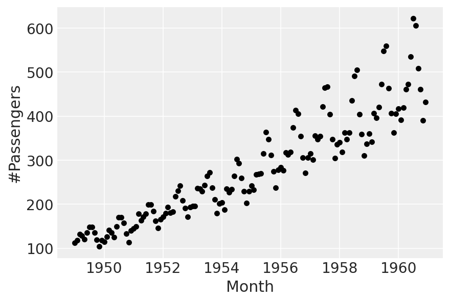
存在增长趋势，以及乘法季节性。我们将拟合线性趋势，并从 Prophet 中“借用”乘法季节性部分。

第 0 部分：缩放数据

首先，我们将时间缩放到 0 到 1 之间

t = (df["Month"] - pd.Timestamp("1900-01-01")).dt.days.to_numpy()
t_min = np.min(t)
t_max = np.max(t)
t = (t - t_min) / (t_max - t_min)

接下来，对于目标变量，我们除以最大值。我们这样做而不是标准化，以便观察值的符号保持不变 - 这对于季节性成分稍后正常工作是必要的。

y = df["#Passengers"].to_numpy()
y_max = np.max(y)
y = y / y_max

第 1 部分：线性趋势

我们现在要拟合的模型将只是

\[\text{Passengers} \sim \alpha + \beta\ \text{time}\]

首先，让我们尝试使用 prophet 设置的默认先验，我们将进行先验预测检查

with pm.Model(check_bounds=False) as linear:
    α = pm.Normal("α", mu=0, sigma=5)
    β = pm.Normal("β", mu=0, sigma=5)
    σ = pm.HalfNormal("σ", sigma=5)
    trend = pm.Deterministic("trend", α + β * t)
    pm.Normal("likelihood", mu=trend, sigma=σ, observed=y)

    linear_prior = pm.sample_prior_predictive()

fig, ax = plt.subplots(nrows=2, ncols=1, sharex=True)
ax[0].plot(
    df["Month"],
    az.extract_dataset(linear_prior, group="prior_predictive", num_samples=100)["likelihood"]
    * y_max,
    color="blue",
    alpha=0.05,
)
df.plot.scatter(x="Month", y="#Passengers", color="k", ax=ax[0])
ax[0].set_title("Prior predictive")
ax[1].plot(
    df["Month"],
    az.extract_dataset(linear_prior, group="prior", num_samples=100)["trend"] * y_max,
    color="blue",
    alpha=0.05,
)
df.plot.scatter(x="Month", y="#Passengers", color="k", ax=ax[1])
ax[1].set_title("Prior trend lines");

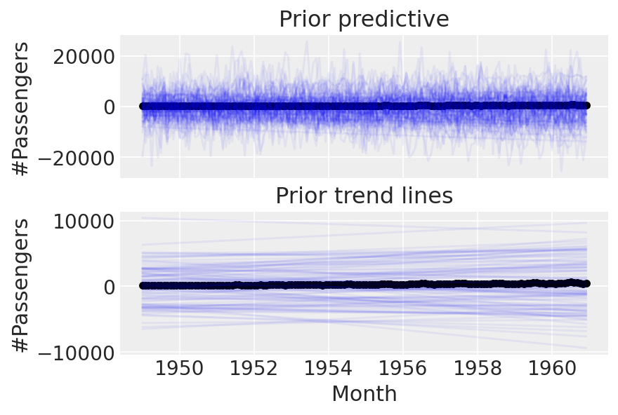
我们可以做得更好。这些先验显然太宽泛了，因为我们最终得到了难以置信的乘客数量。让我们尝试设置更严格的先验。

with pm.Model(check_bounds=False) as linear:
    α = pm.Normal("α", mu=0, sigma=0.5)
    β = pm.Normal("β", mu=0, sigma=0.5)
    σ = pm.HalfNormal("σ", sigma=0.1)
    trend = pm.Deterministic("trend", α + β * t)
    pm.Normal("likelihood", mu=trend, sigma=σ, observed=y)

    linear_prior = pm.sample_prior_predictive(samples=100)

fig, ax = plt.subplots(nrows=2, ncols=1, sharex=True)
ax[0].plot(
    df["Month"],
    az.extract_dataset(linear_prior, group="prior_predictive", num_samples=100)["likelihood"]
    * y_max,
    color="blue",
    alpha=0.05,
)
df.plot.scatter(x="Month", y="#Passengers", color="k", ax=ax[0])
ax[0].set_title("Prior predictive")
ax[1].plot(
    df["Month"],
    az.extract_dataset(linear_prior, group="prior", num_samples=100)["trend"] * y_max,
    color="blue",
    alpha=0.05,
)
df.plot.scatter(x="Month", y="#Passengers", color="k", ax=ax[1])
ax[1].set_title("Prior trend lines");

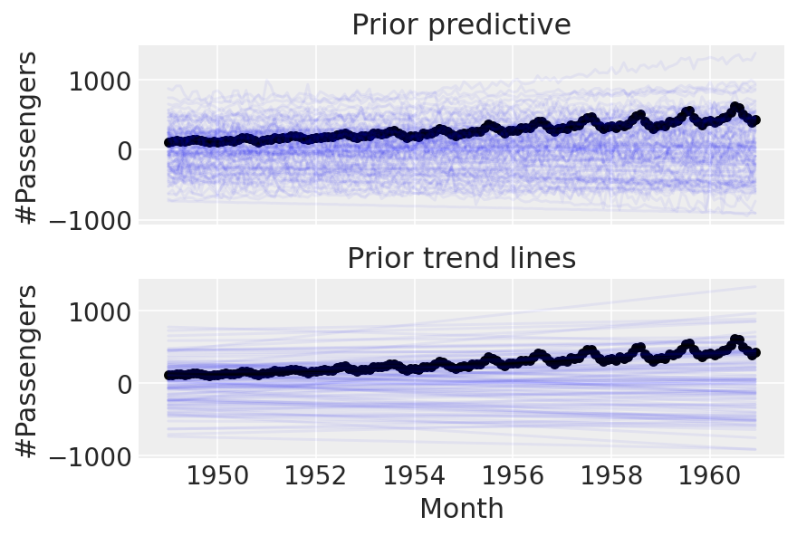
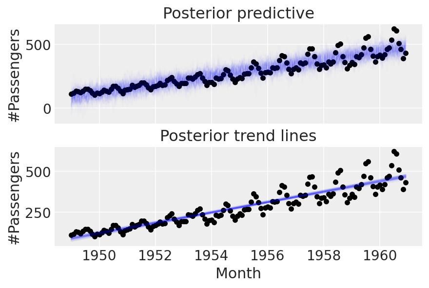
酷。在进行任何更复杂的操作之前，让我们尝试以数据为条件并进行后验预测检查

with linear:
    linear_trace = pm.sample(return_inferencedata=True)
    linear_prior = pm.sample_posterior_predictive(trace=linear_trace)

fig, ax = plt.subplots(nrows=2, ncols=1, sharex=True)
ax[0].plot(
    df["Month"],
    az.extract_dataset(linear_prior, group="posterior_predictive", num_samples=100)["likelihood"]
    * y_max,
    color="blue",
    alpha=0.01,
)
df.plot.scatter(x="Month", y="#Passengers", color="k", ax=ax[0])
ax[0].set_title("Posterior predictive")
ax[1].plot(
    df["Month"],
    az.extract_dataset(linear_trace, group="posterior", num_samples=100)["trend"] * y_max,
    color="blue",
    alpha=0.01,
)
df.plot.scatter(x="Month", y="#Passengers", color="k", ax=ax[1])
ax[1].set_title("Posterior trend lines");

Auto-assigning NUTS sampler...
Initializing NUTS using jitter+adapt_diag...
Multiprocess sampling (4 chains in 4 jobs)
NUTS: [α, β, σ]

100.00% [8000/8000 00:01<00:00 Sampling 4 chains, 0 divergences]

Sampling 4 chains for 1_000 tune and 1_000 draw iterations (4_000 + 4_000 draws total) took 3 seconds.
The acceptance probability does not match the target. It is 0.8849, but should be close to 0.8. Try to increase the number of tuning steps.
The acceptance probability does not match the target. It is 0.8801, but should be close to 0.8. Try to increase the number of tuning steps.

100.00% [4000/4000 00:00<00:00]

第 2 部分：进入季节性

为了模拟季节性，我们将“借用” Prophet 采用的方法 - 请参阅 Prophet 论文 [Taylor and Letham, 2018] 了解详细信息，但其思想是创建一个傅里叶特征矩阵，该矩阵乘以系数向量。由于我们将使用乘法季节性，最终模型将是

\[\text{Passengers} \sim (\alpha + \beta\ \text{time}) (1 + \text{seasonality})\]

n_order = 10
periods = (df["Month"] - pd.Timestamp("1900-01-01")).dt.days / 365.25

fourier_features = pd.DataFrame(
    {
        f"{func}_order_{order}": getattr(np, func)(2 * np.pi * periods * order)
        for order in range(1, n_order + 1)
        for func in ("sin", "cos")
    }
)
fourier_features

	sin_order_1	cos_order_1	sin_order_2	cos_order_2	sin_order_3	cos_order_3	sin_order_4	cos_order_4	sin_order_5	cos_order_5	sin_order_6	cos_order_6	sin_order_7	cos_order_7	sin_order_8	cos_order_8	sin_order_9	cos_order_9	sin_order_10	cos_order_10
0	-0.004301	0.999991	-0.008601	0.999963	-0.012901	0.999917	-0.017202	0.999852	-0.021501	0.999769	-0.025801	0.999667	-0.030100	0.999547	-0.034398	0.999408	-0.038696	0.999251	-0.042993	0.999075
1	0.504648	0.863325	0.871351	0.490660	0.999870	-0.016127	0.855075	-0.518505	0.476544	-0.879150	-0.032249	-0.999480	-0.532227	-0.846602	-0.886721	-0.462305	-0.998830	0.048363	-0.837909	0.545811
2	0.847173	0.531317	0.900235	-0.435405	0.109446	-0.993993	-0.783934	-0.620844	-0.942480	0.334263	-0.217577	0.976043	0.711276	0.702913	0.973402	-0.229104	0.323093	-0.946367	-0.630072	-0.776537
3	0.999639	0.026876	0.053732	-0.998555	-0.996751	-0.080549	-0.107308	0.994226	0.990983	0.133990	0.160575	-0.987024	-0.982352	-0.187043	-0.213377	0.976970	0.970882	0.239557	0.265563	-0.964094
4	0.882712	-0.469915	-0.829598	-0.558361	-0.103031	0.994678	0.926430	-0.376467	-0.767655	-0.640864	-0.204966	0.978769	0.960288	-0.279012	-0.697540	-0.716546	-0.304719	0.952442	0.983924	-0.178587
...	...	...	...	...	...	...	...	...	...	...	...	...	...	...	...	...	...	...	...	...
139	-0.484089	-0.875019	0.847173	0.531317	-0.998497	-0.054805	0.900235	-0.435405	-0.576948	0.816781	0.109446	-0.993993	0.385413	0.922744	-0.783934	-0.620844	0.986501	0.163757	-0.942480	0.334263
140	-0.861693	-0.507430	0.874498	-0.485029	-0.025801	0.999667	-0.848314	-0.529494	0.886721	-0.462305	-0.051584	0.998669	-0.834370	-0.551205	0.898354	-0.439273	-0.077334	0.997005	-0.819871	-0.572548
141	-0.999870	-0.016127	0.032249	-0.999480	0.998830	0.048363	-0.064464	0.997920	-0.996751	-0.080549	0.096613	-0.995322	0.993635	0.112651	-0.128661	0.991689	-0.989485	-0.144636	0.160575	-0.987024
142	-0.869233	0.494403	-0.859503	-0.511131	0.019352	-0.999813	0.878637	-0.477489	0.849450	0.527668	-0.038696	0.999251	-0.887713	0.460397	-0.839080	-0.544008	0.058026	-0.998315	0.896456	-0.443132
143	-0.512055	0.858953	-0.879662	0.475599	-0.999121	-0.041919	-0.836733	-0.547611	-0.438307	-0.898825	0.083764	-0.996486	0.582205	-0.813042	0.916409	-0.400244	0.992099	0.125461	0.787922	0.615774

144 rows × 20 columns

同样，让我们使用默认的 Prophet 先验，看看会发生什么。

coords = {"fourier_features": np.arange(2 * n_order)}
with pm.Model(check_bounds=False, coords=coords) as linear_with_seasonality:
    α = pm.Normal("α", mu=0, sigma=0.5)
    β = pm.Normal("β", mu=0, sigma=0.5)
    σ = pm.HalfNormal("σ", sigma=0.1)
    β_fourier = pm.Normal("β_fourier", mu=0, sigma=10, dims="fourier_features")
    seasonality = pm.Deterministic(
        "seasonality", pm.math.dot(β_fourier, fourier_features.to_numpy().T)
    )
    trend = pm.Deterministic("trend", α + β * t)
    μ = trend * (1 + seasonality)
    pm.Normal("likelihood", mu=μ, sigma=σ, observed=y)

    linear_seasonality_prior = pm.sample_prior_predictive()

fig, ax = plt.subplots(nrows=3, ncols=1, sharex=False, figsize=(8, 6))
ax[0].plot(
    df["Month"],
    az.extract_dataset(linear_seasonality_prior, group="prior_predictive", num_samples=100)[
        "likelihood"
    ]
    * y_max,
    color="blue",
    alpha=0.05,
)
df.plot.scatter(x="Month", y="#Passengers", color="k", ax=ax[0])
ax[0].set_title("Prior predictive")
ax[1].plot(
    df["Month"],
    az.extract_dataset(linear_seasonality_prior, group="prior", num_samples=100)["trend"] * y_max,
    color="blue",
    alpha=0.05,
)
df.plot.scatter(x="Month", y="#Passengers", color="k", ax=ax[1])
ax[1].set_title("Prior trend lines")
ax[2].plot(
    df["Month"].iloc[:12],
    az.extract_dataset(linear_seasonality_prior, group="prior", num_samples=100)["seasonality"][:12]
    * 100,
    color="blue",
    alpha=0.05,
)
ax[2].set_title("Prior seasonality")
ax[2].set_ylabel("Percent change")
formatter = mdates.DateFormatter("%b")
ax[2].xaxis.set_major_formatter(formatter);

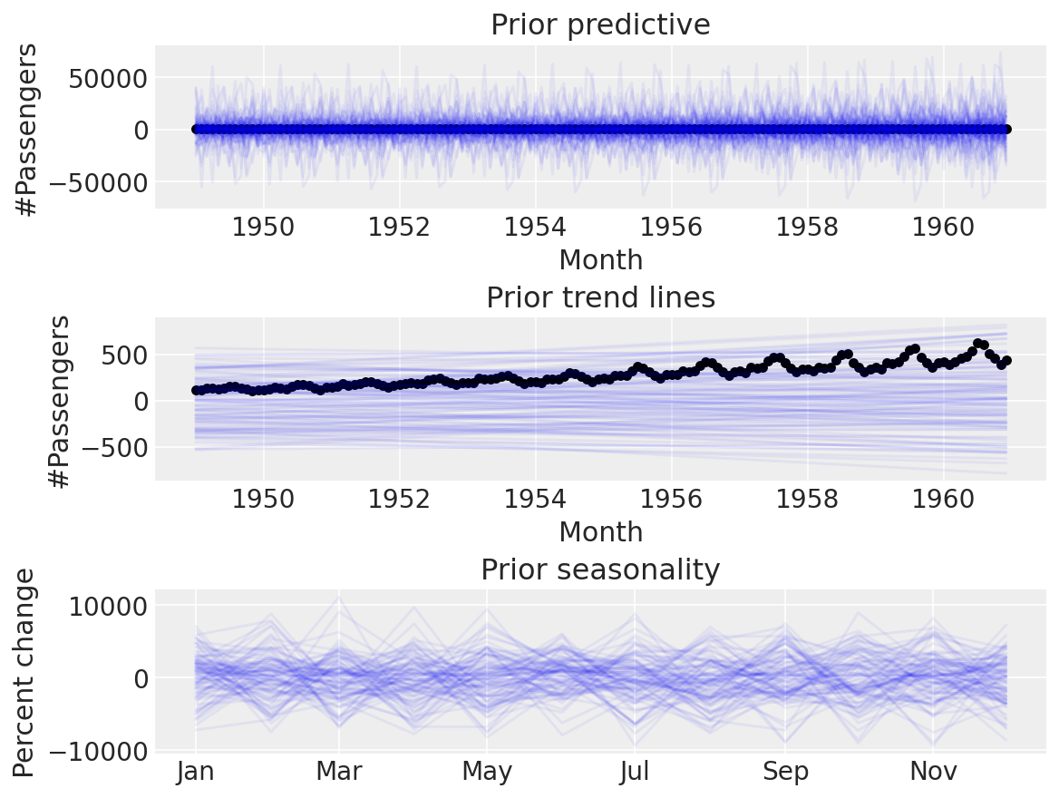
同样，这似乎难以置信。默认的先验对于我们的用例来说太宽泛了，当我们可以进行先验预测检查以设置更合理的先验时，使用它们是没有意义的。让我们尝试一些更窄的先验

coords = {"fourier_features": np.arange(2 * n_order)}
with pm.Model(check_bounds=False, coords=coords) as linear_with_seasonality:
    α = pm.Normal("α", mu=0, sigma=0.5)
    β = pm.Normal("β", mu=0, sigma=0.5)
    trend = pm.Deterministic("trend", α + β * t)

    β_fourier = pm.Normal("β_fourier", mu=0, sigma=0.1, dims="fourier_features")
    seasonality = pm.Deterministic(
        "seasonality", pm.math.dot(β_fourier, fourier_features.to_numpy().T)
    )

    μ = trend * (1 + seasonality)
    σ = pm.HalfNormal("σ", sigma=0.1)
    pm.Normal("likelihood", mu=μ, sigma=σ, observed=y)

    linear_seasonality_prior = pm.sample_prior_predictive()

fig, ax = plt.subplots(nrows=3, ncols=1, sharex=False, figsize=(8, 6))
ax[0].plot(
    df["Month"],
    az.extract_dataset(linear_seasonality_prior, group="prior_predictive", num_samples=100)[
        "likelihood"
    ]
    * y_max,
    color="blue",
    alpha=0.05,
)
df.plot.scatter(x="Month", y="#Passengers", color="k", ax=ax[0])
ax[0].set_title("Prior predictive")
ax[1].plot(
    df["Month"],
    az.extract_dataset(linear_seasonality_prior, group="prior", num_samples=100)["trend"] * y_max,
    color="blue",
    alpha=0.05,
)
df.plot.scatter(x="Month", y="#Passengers", color="k", ax=ax[1])
ax[1].set_title("Prior trend lines")
ax[2].plot(
    df["Month"].iloc[:12],
    az.extract_dataset(linear_seasonality_prior, group="prior", num_samples=100)["seasonality"][:12]
    * 100,
    color="blue",
    alpha=0.05,
)
ax[2].set_title("Prior seasonality")
ax[2].set_ylabel("Percent change")
formatter = mdates.DateFormatter("%b")
ax[2].xaxis.set_major_formatter(formatter);

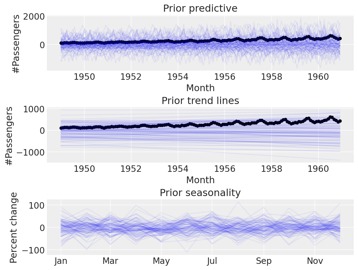
似乎更可信。是时候进行后验预测检查了

with linear_with_seasonality:
    linear_seasonality_trace = pm.sample(return_inferencedata=True)
    linear_seasonality_posterior = pm.sample_posterior_predictive(trace=linear_seasonality_trace)

fig, ax = plt.subplots(nrows=3, ncols=1, sharex=False, figsize=(8, 6))
ax[0].plot(
    df["Month"],
    az.extract_dataset(linear_seasonality_posterior, group="posterior_predictive", num_samples=100)[
        "likelihood"
    ]
    * y_max,
    color="blue",
    alpha=0.05,
)
df.plot.scatter(x="Month", y="#Passengers", color="k", ax=ax[0])
ax[0].set_title("Posterior predictive")
ax[1].plot(
    df["Month"],
    az.extract_dataset(linear_trace, group="posterior", num_samples=100)["trend"] * y_max,
    color="blue",
    alpha=0.05,
)
df.plot.scatter(x="Month", y="#Passengers", color="k", ax=ax[1])
ax[1].set_title("Posterior trend lines")
ax[2].plot(
    df["Month"].iloc[:12],
    az.extract_dataset(linear_seasonality_trace, group="posterior", num_samples=100)["seasonality"][
        :12
    ]
    * 100,
    color="blue",
    alpha=0.05,
)
ax[2].set_title("Posterior seasonality")
ax[2].set_ylabel("Percent change")
formatter = mdates.DateFormatter("%b")
ax[2].xaxis.set_major_formatter(formatter);

Auto-assigning NUTS sampler...
Initializing NUTS using jitter+adapt_diag...
Multiprocess sampling (4 chains in 4 jobs)
NUTS: [α, β, β_fourier, σ]

100.00% [8000/8000 00:15<00:00 Sampling 4 chains, 0 divergences]

Sampling 4 chains for 1_000 tune and 1_000 draw iterations (4_000 + 4_000 draws total) took 16 seconds.

100.00% [4000/4000 00:00<00:00]

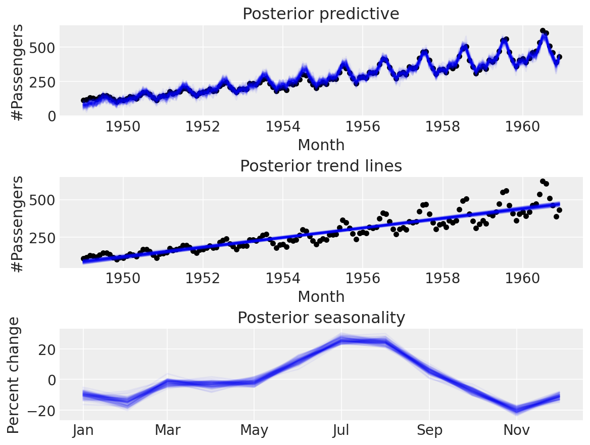
太棒了！

结论

我们看到了如何自己实现类似 Prophet 的模型并将其拟合到航空乘客数据集。Prophet 是一个很棒的库，对社区有积极的意义，但是通过自己实现它，我们可以采用我们认为与我们的问题相关的任何组件，自定义它们，并执行贝叶斯工作流程 [Gelman et al., 2020]）。下次您遇到时间序列问题时，我希望您尝试实现自己的概率模型，而不是将 Prophet 用作参数可调的“黑匣子”。

作为参考，您可能还想查看

• TimeSeeers，一个基于 Facebook Prophet 的分层贝叶斯时间序列模型，用 PyMC3 编写

• PM-Prophet，一个基于 Pymc3 的通用时间序列预测和分解库，灵感来自 Facebook Prophet

作者

• 由 Marco Gorelli 于 2021 年 6 月创作 (pymc-examples#183)

• 由 Danh Phan 于 2022 年 5 月更新 (pymc-examples#320)

参考文献

[1] (1,2)

Andrew Gelman, Aki Vehtari, Daniel Simpson, Charles C Margossian, Bob Carpenter, Yuling Yao, Lauren Kennedy, Jonah Gabry, Paul-Christian Bürkner, 和 Martin Modrák. Bayesian workflow. arXiv preprint arXiv:2011.01808, 2020. URL: https://arxiv.org/abs/2011.01808.

[2] (1,2)

Sean J Taylor 和 Benjamin Letham. Forecasting at scale. The American Statistician, 72(1):37–45, 2018. URL: https://peerj.com/preprints/3190/.

%load_ext watermark
%watermark -n -u -v -iv -w -p pytensor,aeppl,xarray

Last updated: Sun May 29 2022

Python implementation: CPython
Python version       : 3.9.12
IPython version      : 8.3.0

pytensor: 2.6.2
aeppl : 0.0.28
xarray: 2022.3.0

arviz     : 0.12.1
matplotlib: 3.5.2
pymc      : 4.0.0b6
numpy     : 1.22.4
pandas    : 1.4.2

Watermark: 2.3.0

许可声明

此示例库中的所有笔记本均根据 MIT 许可证 提供，该许可证允许修改和再分发用于任何用途，前提是保留版权和许可证声明。

引用 PyMC 示例

要引用此笔记本，请使用 Zenodo 为 pymc-examples 存储库提供的 DOI。

重要提示

许多笔记本都改编自其他来源：博客、书籍……在这种情况下，您也应该引用原始来源。

另请记住引用您的代码使用的相关库。

这是一个 bibtex 中的引用模板

@incollection{citekey,
  author    = "<notebook authors, see above>",
  title     = "<notebook title>",
  editor    = "PyMC Team",
  booktitle = "PyMC examples",
  doi       = "10.5281/zenodo.5654871"
}

一旦渲染，它可能看起来像