使用结构自回归时间序列进行预测#

贝叶斯结构时间序列模型是了解任何观测时间序列数据内在结构的有趣方法。它还使我们能够向前投影隐含的预测分布，从而为我们提供预测问题的另一种视角。我们可以将迄今为止观察到的时间序列数据的学习特征视为对同一指标的未实现未来状态结构的参考。

在本笔记本中，我们将了解如何拟合和预测一系列自回归结构时间序列模型，以及重要的是，如何预测模型的未来观测值。

import arviz as az
import numpy as np
import pandas as pd
import pymc as pm

from matplotlib import pyplot as plt

RANDOM_SEED = 8929
rng = np.random.default_rng(RANDOM_SEED)
az.style.use("arviz-darkgrid")

生成伪自回归数据#

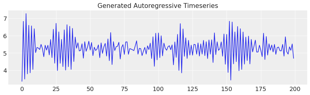
首先，我们将生成一个简单的自回归时间序列。我们将展示如何指定一个模型来拟合这些数据，然后向数据添加一些复杂性，并展示如何使用自回归模型捕获这些复杂性，并用于预测未来的形状。

def simulate_ar(intercept, coef1, coef2, noise=0.3, *, warmup=10, steps=200):
    # We sample some extra warmup steps, to let the AR process stabilize
    draws = np.zeros(warmup + steps)
    # Initialize first draws at intercept
    draws[:2] = intercept
    for step in range(2, warmup + steps):
        draws[step] = (
            intercept
            + coef1 * draws[step - 1]
            + coef2 * draws[step - 2]
            + np.random.normal(0, noise)
        )
    # Discard the warmup draws
    return draws[warmup:]


# True parameters of the AR process
ar1_data = simulate_ar(10, -0.9, 0)

fig, ax = plt.subplots(figsize=(10, 3))
ax.set_title("Generated Autoregressive Timeseries", fontsize=15)
ax.plot(ar1_data);

../_images/a72e7a83bd44131c4c544f52c3de3fb4df7aaf7e9b41e35f5981c9868c69b765.png

指定模型#

我们将逐步介绍模型，然后将该模式概括为一个函数，该函数可用于采用日益复杂的组件结构组合。

## Set up a dictionary for the specification of our priors
## We set up the dictionary to specify size of the AR coefficients in
## case we want to vary the AR lags.
priors = {
    "coefs": {"mu": [10, 0.2], "sigma": [0.1, 0.1], "size": 2},
    "sigma": 8,
    "init": {"mu": 9, "sigma": 0.1, "size": 1},
}

## Initialise the model
with pm.Model() as AR:
    pass

## Define the time interval for fitting the data
t_data = list(range(len(ar1_data)))
## Add the time interval as a mutable coordinate to the model to allow for future predictions
AR.add_coord("obs_id", t_data, mutable=True)

with AR:
    ## Data containers to enable prediction
    t = pm.MutableData("t", t_data, dims="obs_id")
    y = pm.MutableData("y", ar1_data, dims="obs_id")

    # The first coefficient will be the constant term but we need to set priors for each coefficient in the AR process
    coefs = pm.Normal("coefs", priors["coefs"]["mu"], priors["coefs"]["sigma"])
    sigma = pm.HalfNormal("sigma", priors["sigma"])
    # We need one init variable for each lag, hence size is variable too
    init = pm.Normal.dist(
        priors["init"]["mu"], priors["init"]["sigma"], size=priors["init"]["size"]
    )
    # Steps of the AR model minus the lags required
    ar1 = pm.AR(
        "ar",
        coefs,
        sigma=sigma,
        init_dist=init,
        constant=True,
        steps=t.shape[0] - (priors["coefs"]["size"] - 1),
        dims="obs_id",
    )

    # The Likelihood
    outcome = pm.Normal("likelihood", mu=ar1, sigma=sigma, observed=y, dims="obs_id")
    ## Sampling
    idata_ar = pm.sample_prior_predictive()
    idata_ar.extend(pm.sample(2000, random_seed=100, target_accept=0.95))
    idata_ar.extend(pm.sample_posterior_predictive(idata_ar))

Sampling: [ar, coefs, likelihood, sigma]
Auto-assigning NUTS sampler...
Initializing NUTS using jitter+adapt_diag...
Multiprocess sampling (4 chains in 4 jobs)
NUTS: [coefs, sigma, ar]

100.00% [12000/12000 00:26<00:00 采样 4 条链，0 个发散]

Sampling 4 chains for 1_000 tune and 2_000 draw iterations (4_000 + 8_000 draws total) took 46 seconds.
Sampling: [likelihood]

100.00% [8000/8000 00:00<00:00]

让我们用盘式符号检查模型结构，然后检查收敛诊断。

az.plot_trace(idata_ar, figsize=(10, 6), kind="rank_vlines");

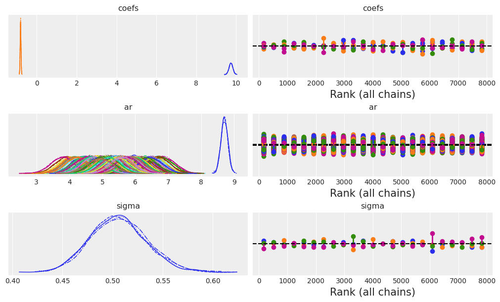
../_images/d89679b6818cb9e3a3ec9c556a88886cb17d4cd46eb9d20281216a1863a6d8f2.png

接下来，我们将检查 AR 系数和 sigma 项的摘要估计。

az.summary(idata_ar, var_names=["~ar"])

	均值	标准差	hdi_3%	hdi_97%	mcse_mean	mcse_sd	ess_bulk	ess_tail	r_hat
coefs[0]	9.744	0.094	9.555	9.911	0.001	0.001	13107.0	6200.0	1.0
coefs[1]	-0.815	0.021	-0.854	-0.776	0.000	0.000	9141.0	5792.0	1.0
sigma	0.506	0.028	0.453	0.557	0.001	0.000	2965.0	5254.0	1.0

我们可以在这里看到，模型拟合相当正确地估计了数据生成过程的真实参数。如果我们绘制后验 ar 分布与我们的观测数据，我们也可以看到这一点。

fig, ax = plt.subplots(figsize=(10, 4))
idata_ar.posterior.ar.mean(["chain", "draw"]).plot(ax=ax, label="Posterior Mean AR level")
ax.plot(ar1_data, "o", color="black", markersize=2, label="Observed Data")
ax.legend()
ax.set_title("Fitted AR process\nand observed data");

../_images/9bb5fa7766e0dfa6c0375e9c37f68c925411d36bec022d5264ca732b075e14bf.png

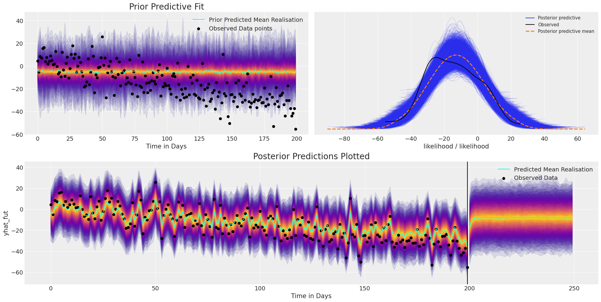
检查模型拟合和预测#

我们可以查看标准后验预测拟合，但由于我们的数据是时间序列数据，因此我们还必须查看后验预测分布的抽取如何随时间变化。

def plot_fits(idata_ar, idata_preds):
    palette = "plasma"
    cmap = plt.get_cmap(palette)
    percs = np.linspace(51, 99, 100)
    colors = (percs - np.min(percs)) / (np.max(percs) - np.min(percs))
    mosaic = """AABB
                CCCC"""
    fig, axs = plt.subplot_mosaic(mosaic, sharex=False, figsize=(20, 10))
    axs = [axs[k] for k in axs.keys()]
    for i, p in enumerate(percs[::-1]):
        upper = np.percentile(
            az.extract_dataset(idata_ar, group="prior_predictive", num_samples=1000)["likelihood"],
            p,
            axis=1,
        )
        lower = np.percentile(
            az.extract_dataset(idata_ar, group="prior_predictive", num_samples=1000)["likelihood"],
            100 - p,
            axis=1,
        )
        color_val = colors[i]
        axs[0].fill_between(
            x=idata_ar["constant_data"]["t"],
            y1=upper.flatten(),
            y2=lower.flatten(),
            color=cmap(color_val),
            alpha=0.1,
        )

    axs[0].plot(
        az.extract_dataset(idata_ar, group="prior_predictive", num_samples=1000)["likelihood"].mean(
            axis=1
        ),
        color="cyan",
        label="Prior Predicted Mean Realisation",
    )

    axs[0].scatter(
        x=idata_ar["constant_data"]["t"],
        y=idata_ar["constant_data"]["y"],
        color="k",
        label="Observed Data points",
    )
    axs[0].set_title("Prior Predictive Fit", fontsize=20)
    axs[0].legend()

    for i, p in enumerate(percs[::-1]):
        upper = np.percentile(
            az.extract_dataset(idata_preds, group="predictions", num_samples=1000)["likelihood"],
            p,
            axis=1,
        )
        lower = np.percentile(
            az.extract_dataset(idata_preds, group="predictions", num_samples=1000)["likelihood"],
            100 - p,
            axis=1,
        )
        color_val = colors[i]
        axs[2].fill_between(
            x=idata_preds["predictions_constant_data"]["t"],
            y1=upper.flatten(),
            y2=lower.flatten(),
            color=cmap(color_val),
            alpha=0.1,
        )

        upper = np.percentile(
            az.extract_dataset(idata_preds, group="predictions", num_samples=1000)["yhat_fut"],
            p,
            axis=1,
        )
        lower = np.percentile(
            az.extract_dataset(idata_preds, group="predictions", num_samples=1000)["yhat_fut"],
            100 - p,
            axis=1,
        )
        color_val = colors[i]
        axs[2].fill_between(
            x=idata_preds["predictions"].coords["obs_id_fut"].data,
            y1=upper.flatten(),
            y2=lower.flatten(),
            color=cmap(color_val),
            alpha=0.1,
        )

    axs[2].plot(
        az.extract_dataset(idata_preds, group="predictions", num_samples=1000)["likelihood"].mean(
            axis=1
        ),
        color="cyan",
    )
    idata_preds.predictions.yhat_fut.mean(["chain", "draw"]).plot(
        ax=axs[2], color="cyan", label="Predicted Mean Realisation"
    )
    axs[2].scatter(
        x=idata_ar["constant_data"]["t"],
        y=idata_ar["constant_data"]["y"],
        color="k",
        label="Observed Data",
    )
    axs[2].set_title("Posterior Predictions Plotted", fontsize=20)
    axs[2].axvline(np.max(idata_ar["constant_data"]["t"]), color="black")
    axs[2].legend()
    axs[2].set_xlabel("Time in Days")
    axs[0].set_xlabel("Time in Days")
    az.plot_ppc(idata_ar, ax=axs[1])


plot_fits(idata_ar, idata_preds)

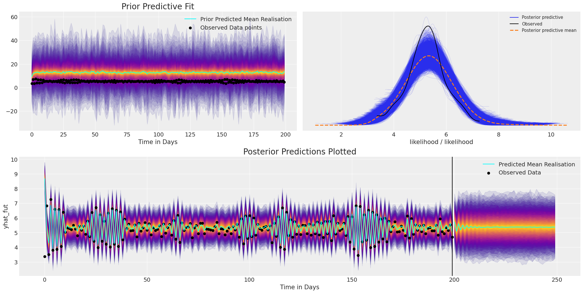
../_images/50c1547d7d5179e56668f96f85b4fa8923caf69edefeea7a5fcfed87168d99d5.png

在这里我们可以看到，尽管模型收敛并且最终对现有数据进行了合理的拟合，并且对未来值进行了**合理的预测**。但是，由于自回归函数的复合逻辑，我们在先验规范中设置得非常差，允许了极其广泛的值范围。因此，能够使用先验预测检查来检查和定制您的模型非常重要。

其次，平均预测未能捕获任何持久的结构，而是迅速衰减到稳定的基线。为了解决这些短暂的预测，我们可以为我们的模型添加更多结构，但首先，让我们使情况复杂化。

使情况复杂化#

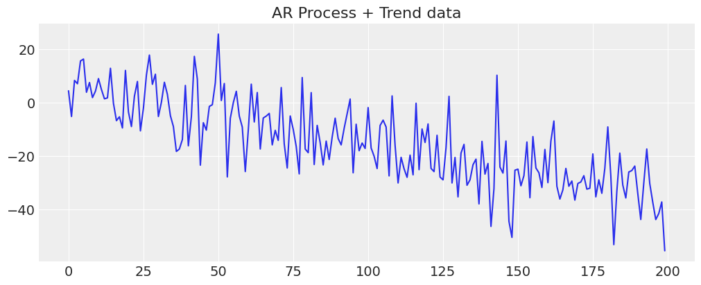
通常，我们的数据将涉及多个潜在过程，并且可能具有更复杂的因素来驱动结果。为了看到这样一个复杂性，让我们在数据中添加一个趋势。通过为我们的预测添加更多结构，我们是在告诉我们的模型，我们期望某些模式或趋势在未来的数据中保持不变。添加哪些结构的选择由富有创造力的建模者自行决定 - 在这里我们将演示一些简单的示例。

y_t = -0.3 + np.arange(200) * -0.2 + np.random.normal(0, 10, 200)
y_t = y_t + ar1_data

fig, ax = plt.subplots(figsize=(10, 4))
ax.plot(y_t)
ax.set_title("AR Process + Trend data");

../_images/60f92ba6eb44c8cdab53d78b81da6e84c3d3e8cc024556a1b6e60f5897c0ee3a.png

将我们的模型包装成函数#

def make_latent_AR_model(ar_data, priors, prediction_steps=250, full_sample=True, samples=2000):
    with pm.Model() as AR:
        pass

    t_data = list(range(len(ar_data)))
    AR.add_coord("obs_id", t_data, mutable=True)

    with AR:
        ## Data containers to enable prediction
        t = pm.MutableData("t", t_data, dims="obs_id")
        y = pm.MutableData("y", ar_data, dims="obs_id")
        # The first coefficient will be the intercept term
        coefs = pm.Normal("coefs", priors["coefs"]["mu"], priors["coefs"]["sigma"])
        sigma = pm.HalfNormal("sigma", priors["sigma"])
        # We need one init variable for each lag, hence size is variable too
        init = pm.Normal.dist(
            priors["init"]["mu"], priors["init"]["sigma"], size=priors["init"]["size"]
        )
        # Steps of the AR model minus the lags required given specification
        ar1 = pm.AR(
            "ar",
            coefs,
            sigma=sigma,
            init_dist=init,
            constant=True,
            steps=t.shape[0] - (priors["coefs"]["size"] - 1),
            dims="obs_id",
        )

        # The Likelihood
        outcome = pm.Normal("likelihood", mu=ar1, sigma=sigma, observed=y, dims="obs_id")
        ## Sampling
        idata_ar = pm.sample_prior_predictive()
        if full_sample:
            idata_ar.extend(pm.sample(samples, random_seed=100, target_accept=0.95))
            idata_ar.extend(pm.sample_posterior_predictive(idata_ar))
        else:
            return idata_ar

    n = prediction_steps - ar_data.shape[0]

    with AR:
        AR.add_coords({"obs_id_fut_1": range(ar1_data.shape[0] - 1, 250, 1)})
        AR.add_coords({"obs_id_fut": range(ar1_data.shape[0], 250, 1)})
        # condition on the learned values of the AR process
        # initialise the future AR process precisely at the last observed value in the AR process
        # using the special feature of the dirac delta distribution to be 0 probability everywhere else.
        ar1_fut = pm.AR(
            "ar1_fut",
            init_dist=pm.DiracDelta.dist(ar1[..., -1]),
            rho=coefs,
            sigma=sigma,
            constant=True,
            dims="obs_id_fut_1",
        )
        yhat_fut = pm.Normal("yhat_fut", mu=ar1_fut[1:], sigma=sigma, dims="obs_id_fut")
        # use the updated values and predict outcomes and probabilities:
        idata_preds = pm.sample_posterior_predictive(
            idata_ar, var_names=["likelihood", "yhat_fut"], predictions=True, random_seed=100
        )

    return idata_ar, idata_preds, AR

接下来，我们将循环遍历一些先验规范，以显示它如何影响先验预测分布，即如果我们从先验指定的模型中向前采样，我们的结果的隐含分布。

priors_0 = {
    "coefs": {"mu": [-4, 0.2], "sigma": 0.1, "size": 2},
    "sigma": 8,
    "init": {"mu": 9, "sigma": 0.1, "size": 1},
}

priors_1 = {
    "coefs": {"mu": [-2, 0.2], "sigma": 0.1, "size": 2},
    "sigma": 12,
    "init": {"mu": 8, "sigma": 0.1, "size": 1},
}

priors_2 = {
    "coefs": {"mu": [0, 0.2], "sigma": 0.1, "size": 2},
    "sigma": 15,
    "init": {"mu": 8, "sigma": 0.1, "size": 1},
}

models = {}
for i, p in enumerate([priors_0, priors_1, priors_2]):
    models[i] = {}
    idata = make_latent_AR_model(y_t, p, full_sample=False)
    models[i]["idata"] = idata

Sampling: [ar, coefs, likelihood, sigma]
Sampling: [ar, coefs, likelihood, sigma]
Sampling: [ar, coefs, likelihood, sigma]

fig, axs = plt.subplots(1, 3, figsize=(10, 4), sharey=True)
axs = axs.flatten()
for i, p in zip(range(3), [priors_0, priors_1, priors_2]):
    axs[i].plot(
        az.extract_dataset(models[i]["idata"], group="prior_predictive", num_samples=100)[
            "likelihood"
        ],
        color="blue",
        alpha=0.1,
    )
    axs[i].plot(y_t, "o", color="black", markersize=2)
    axs[i].set_title(
        "$y_{t+1}$" + f'= N({p["coefs"]["mu"][0]} + {p["coefs"]["mu"][1]}y$_t$, {p["sigma"]})'
    )
plt.suptitle("Prior Predictive Specifications", fontsize=20);

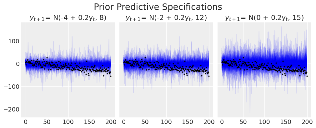
../_images/382fa52b8854574ad31a5a7213a0d0859dbd3a682d00e4da19051733e948e75b.png

我们可以看到模型在捕获趋势线的方式上遇到的困难。增加模型的变异性永远不会捕捉到我们知道存在于数据中的方向模式。

priors_0 = {
    "coefs": {"mu": [-4, 0.2], "sigma": [0.5, 0.03], "size": 2},
    "sigma": 8,
    "init": {"mu": -4, "sigma": 0.1, "size": 1},
}

idata_no_trend, preds_no_trend, model = make_latent_AR_model(y_t, priors_0)

Sampling: [ar, coefs, likelihood, sigma]
Auto-assigning NUTS sampler...
Initializing NUTS using jitter+adapt_diag...
Multiprocess sampling (4 chains in 4 jobs)
NUTS: [coefs, sigma, ar]

100.00% [12000/12000 00:22<00:00 采样 4 条链，0 个发散]

Sampling 4 chains for 1_000 tune and 2_000 draw iterations (4_000 + 8_000 draws total) took 49 seconds.
Sampling: [likelihood]

100.00% [8000/8000 00:00<00:00]

Sampling: [ar1_fut, likelihood, yhat_fut]

100.00% [8000/8000 00:29<00:00]

plot_fits(idata_no_trend, preds_no_trend)

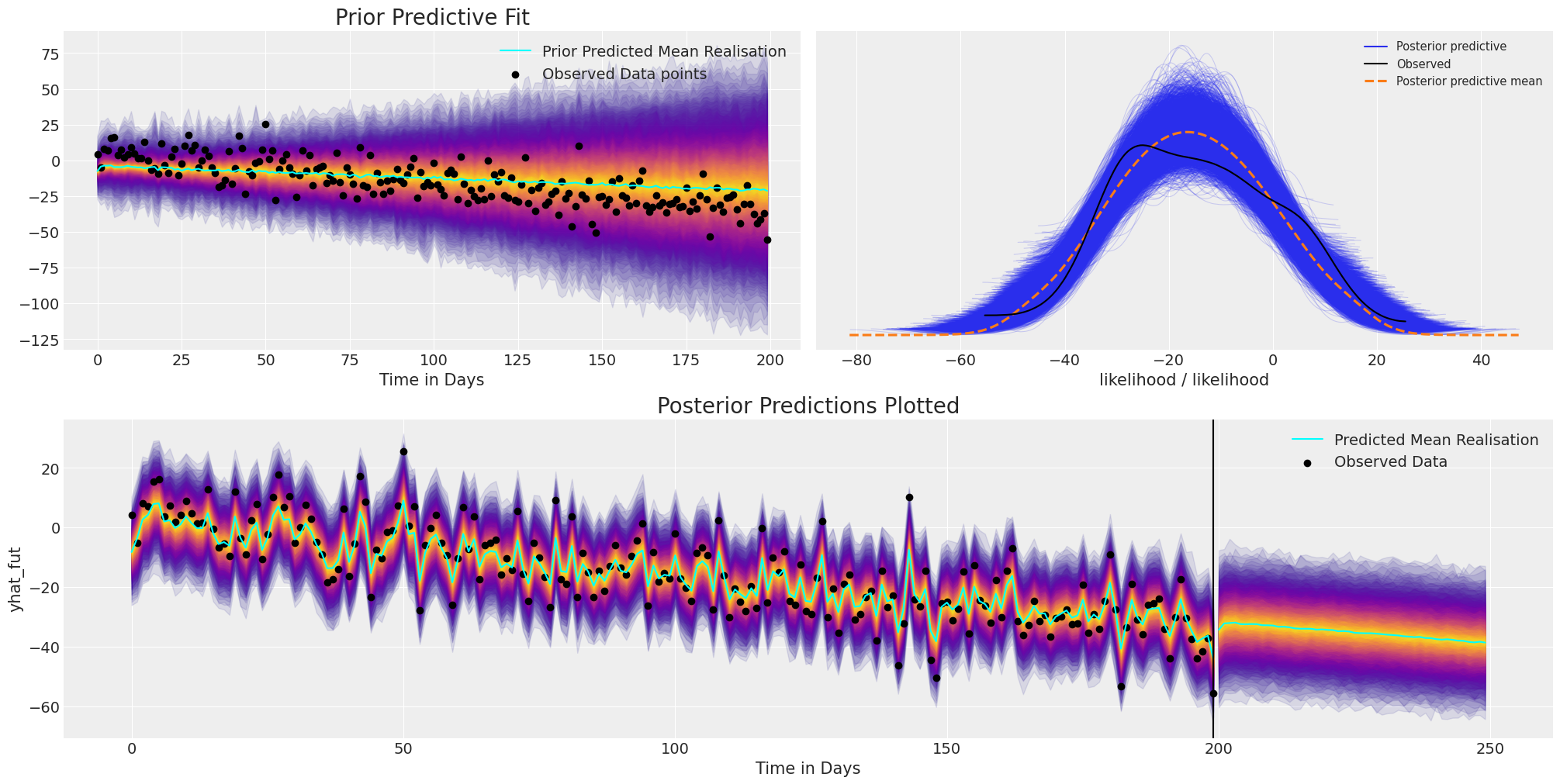
../_images/964c239d241b2d5fe552c598f317302019331701e8d254575779447c685e984a.png

使用此模型进行预测在某种程度上是徒劳的，因为虽然模型拟合可以很好地调整观测数据，但它完全未能捕获数据中的结构趋势。因此，如果没有一些结构约束，当我们试图使用这个简单的 AR 模型进行预测时，它会非常迅速地恢复到平均水平预测。

指定趋势模型#

我们将定义一个模型来解释数据中的趋势，并将此趋势与自回归组件在加性模型中结合起来。同样，该模型与以前的模型非常相似，但现在我们添加了额外的潜在特征。这些特征将以简单的加性组合方式组合，但如果适合我们的模型，我们可以在这里更具创造性。

def make_latent_AR_trend_model(
    ar_data, priors, prediction_steps=250, full_sample=True, samples=2000
):
    with pm.Model() as AR:
        pass

    t_data = list(range(len(ar_data)))
    AR.add_coord("obs_id", t_data, mutable=True)

    with AR:
        ## Data containers to enable prediction
        t = pm.MutableData("t", t_data, dims="obs_id")
        y = pm.MutableData("y", ar_data, dims="obs_id")
        # The first coefficient will be the intercept term
        coefs = pm.Normal("coefs", priors["coefs"]["mu"], priors["coefs"]["sigma"])
        sigma = pm.HalfNormal("sigma", priors["sigma"])
        # We need one init variable for each lag, hence size is variable too
        init = pm.Normal.dist(
            priors["init"]["mu"], priors["init"]["sigma"], size=priors["init"]["size"]
        )
        # Steps of the AR model minus the lags required given specification
        ar1 = pm.AR(
            "ar",
            coefs,
            sigma=sigma,
            init_dist=init,
            constant=True,
            steps=t.shape[0] - (priors["coefs"]["size"] - 1),
            dims="obs_id",
        )

        ## Priors for the linear trend component
        alpha = pm.Normal("alpha", priors["alpha"]["mu"], priors["alpha"]["sigma"])
        beta = pm.Normal("beta", priors["beta"]["mu"], priors["beta"]["sigma"])
        trend = pm.Deterministic("trend", alpha + beta * t, dims="obs_id")

        mu = ar1 + trend

        # The Likelihood
        outcome = pm.Normal("likelihood", mu=mu, sigma=sigma, observed=y, dims="obs_id")
        ## Sampling
        idata_ar = pm.sample_prior_predictive()
        if full_sample:
            idata_ar.extend(pm.sample(samples, random_seed=100, target_accept=0.95))
            idata_ar.extend(pm.sample_posterior_predictive(idata_ar))
        else:
            return idata_ar

    n = prediction_steps - ar_data.shape[0]

    with AR:
        AR.add_coords({"obs_id_fut_1": range(ar1_data.shape[0] - 1, prediction_steps, 1)})
        AR.add_coords({"obs_id_fut": range(ar1_data.shape[0], prediction_steps, 1)})
        t_fut = pm.MutableData("t_fut", list(range(ar1_data.shape[0], prediction_steps, 1)))
        # condition on the learned values of the AR process
        # initialise the future AR process precisely at the last observed value in the AR process
        # using the special feature of the dirac delta distribution to be 0 probability everywhere else.
        ar1_fut = pm.AR(
            "ar1_fut",
            init_dist=pm.DiracDelta.dist(ar1[..., -1]),
            rho=coefs,
            sigma=sigma,
            constant=True,
            dims="obs_id_fut_1",
        )
        trend = pm.Deterministic("trend_fut", alpha + beta * t_fut, dims="obs_id_fut")
        mu = ar1_fut[1:] + trend

        yhat_fut = pm.Normal("yhat_fut", mu=mu, sigma=sigma, dims="obs_id_fut")
        # use the updated values and predict outcomes and probabilities:
        idata_preds = pm.sample_posterior_predictive(
            idata_ar, var_names=["likelihood", "yhat_fut"], predictions=True, random_seed=100
        )

    return idata_ar, idata_preds, AR

我们将通过指定负趋势的先验和标准差范围来拟合此模型，以符合数据漂移的方向。

priors_0 = {
    "coefs": {"mu": [0.2, 0.2], "sigma": [0.5, 0.03], "size": 2},
    "alpha": {"mu": -4, "sigma": 0.1},
    "beta": {"mu": -0.1, "sigma": 0.2},
    "sigma": 8,
    "init": {"mu": -4, "sigma": 0.1, "size": 1},
}


idata_trend, preds_trend, model = make_latent_AR_trend_model(y_t, priors_0, full_sample=True)

Sampling: [alpha, ar, beta, coefs, likelihood, sigma]
Auto-assigning NUTS sampler...
Initializing NUTS using jitter+adapt_diag...
Multiprocess sampling (4 chains in 4 jobs)
NUTS: [coefs, sigma, ar, alpha, beta]

100.00% [12000/12000 00:33<00:00 采样 4 条链，0 个发散]

Sampling 4 chains for 1_000 tune and 2_000 draw iterations (4_000 + 8_000 draws total) took 57 seconds.
Sampling: [likelihood]

100.00% [8000/8000 00:00<00:00]

Sampling: [ar1_fut, likelihood, yhat_fut]

100.00% [8000/8000 00:30<00:00]

pm.model_to_graphviz(model)

../_images/734d82652185212052440dcf2a189d4862d7b6bf22f4bd4e1f64ff5d9032a80a.svg

我们可以使用盘式符号更清楚地看到结构，并且这种额外的结构有助于适当地拟合时间序列数据的方向趋势。

plot_fits(idata_trend, preds_trend);

../_images/722bf61555339ad1f1329e95ebd305407a4d42c1516adc7d792ae0757a5c1d1e.png

az.summary(idata_trend, var_names=["coefs", "sigma", "alpha", "beta"])

	均值	标准差	hdi_3%	hdi_97%	mcse_mean	mcse_sd	ess_bulk	ess_tail	r_hat
coefs[0]	1.086	0.475	0.220	2.006	0.010	0.007	2482.0	4278.0	1.0
coefs[1]	0.210	0.029	0.156	0.264	0.000	0.000	7296.0	5931.0	1.0
sigma	7.557	0.389	6.841	8.284	0.007	0.005	3332.0	4817.0	1.0
alpha	-3.969	0.099	-4.171	-3.794	0.001	0.001	9220.0	5606.0	1.0
beta	-0.145	0.009	-0.161	-0.128	0.000	0.000	1785.0	3995.0	1.0

进一步使情况复杂化#

接下来，我们将向数据添加季节性成分，并了解如何使用贝叶斯结构时间序列模型恢复数据的这一方面。同样，这是因为在现实中，我们的数据通常是多种收敛影响的结果。这些影响可以在加性贝叶斯结构模型中捕获，在加性贝叶斯结构模型中，我们的推断模型确保我们为每个组件分配适当的权重。

t_data = list(range(200))
n_order = 10
periods = np.array(t_data) / 7

fourier_features = pd.DataFrame(
    {
        f"{func}_order_{order}": getattr(np, func)(2 * np.pi * periods * order)
        for order in range(1, n_order + 1)
        for func in ("sin", "cos")
    }
)

y_t_s = y_t + 20 * fourier_features["sin_order_1"]

fig, ax = plt.subplots(figsize=(10, 4))
ax.plot(y_t_s)
ax.set_title("AR + Trend + Seasonality");

../_images/285e345411293af1986d5240b1c81a77d7681751d8dda5c72f03705d6f760f51.png

拟合此模型的关键是理解我们现在正在传入合成傅里叶特征，以帮助解释季节性效应。这之所以有效，是因为（粗略地说）我们试图使用正弦波和余弦波的加权组合来拟合复杂的振荡现象。因此，我们像在回归模型中添加任何其他特征变量一样添加这些正弦波和余弦波。

但是，由于我们使用此加权和来拟合观测数据，因此模型现在**也**期望在预测步骤中使用这些合成特征的线性组合。因此，即使在未来，我们也需要能够提供这些特征。对于我们可能想要添加的任何其他类型的预测特征（例如，星期几、节假日虚拟变量或任何其他特征）而言，这一事实仍然是关键。如果需要特征来拟合观测数据，则预测步骤中也必须提供该特征。

指定趋势 + 季节性模型#

def make_latent_AR_trend_seasonal_model(
    ar_data, ff, priors, prediction_steps=250, full_sample=True, samples=2000
):
    with pm.Model() as AR:
        pass

    ff = ff.to_numpy().T
    t_data = list(range(len(ar_data)))
    AR.add_coord("obs_id", t_data, mutable=True)
    ## The fourier features must be mutable to allow for addition fourier features to be
    ## passed in the prediction step.
    AR.add_coord("fourier_features", np.arange(len(ff)), mutable=True)

    with AR:
        ## Data containers to enable prediction
        t = pm.MutableData("t", t_data, dims="obs_id")
        y = pm.MutableData("y", ar_data, dims="obs_id")
        # The first coefficient will be the intercept term
        coefs = pm.Normal("coefs", priors["coefs"]["mu"], priors["coefs"]["sigma"])
        sigma = pm.HalfNormal("sigma", priors["sigma"])
        # We need one init variable for each lag, hence size is variable too
        init = pm.Normal.dist(
            priors["init"]["mu"], priors["init"]["sigma"], size=priors["init"]["size"]
        )
        # Steps of the AR model minus the lags required given specification
        ar1 = pm.AR(
            "ar",
            coefs,
            sigma=sigma,
            init_dist=init,
            constant=True,
            steps=t.shape[0] - (priors["coefs"]["size"] - 1),
            dims="obs_id",
        )

        ## Priors for the linear trend component
        alpha = pm.Normal("alpha", priors["alpha"]["mu"], priors["alpha"]["sigma"])
        beta = pm.Normal("beta", priors["beta"]["mu"], priors["beta"]["sigma"])
        trend = pm.Deterministic("trend", alpha + beta * t, dims="obs_id")

        ## Priors for seasonality
        beta_fourier = pm.Normal(
            "beta_fourier",
            mu=priors["beta_fourier"]["mu"],
            sigma=priors["beta_fourier"]["sigma"],
            dims="fourier_features",
        )
        fourier_terms = pm.MutableData("fourier_terms", ff)
        seasonality = pm.Deterministic(
            "seasonality", pm.math.dot(beta_fourier, fourier_terms), dims="obs_id"
        )

        mu = ar1 + trend + seasonality

        # The Likelihood
        outcome = pm.Normal("likelihood", mu=mu, sigma=sigma, observed=y, dims="obs_id")
        ## Sampling
        idata_ar = pm.sample_prior_predictive()
        if full_sample:
            idata_ar.extend(pm.sample(samples, random_seed=100, target_accept=0.95))
            idata_ar.extend(pm.sample_posterior_predictive(idata_ar))
        else:
            return idata_ar

    n = prediction_steps - ar_data.shape[0]
    n_order = 10
    periods = (ar_data.shape[0] + np.arange(n)) / 7

    fourier_features_new = pd.DataFrame(
        {
            f"{func}_order_{order}": getattr(np, func)(2 * np.pi * periods * order)
            for order in range(1, n_order + 1)
            for func in ("sin", "cos")
        }
    )

    with AR:
        AR.add_coords({"obs_id_fut_1": range(ar1_data.shape[0] - 1, prediction_steps, 1)})
        AR.add_coords({"obs_id_fut": range(ar1_data.shape[0], prediction_steps, 1)})
        t_fut = pm.MutableData(
            "t_fut", list(range(ar1_data.shape[0], prediction_steps, 1)), dims="obs_id_fut"
        )
        ff_fut = pm.MutableData("ff_fut", fourier_features_new.to_numpy().T)
        # condition on the learned values of the AR process
        # initialise the future AR process precisely at the last observed value in the AR process
        # using the special feature of the dirac delta distribution to be 0 probability everywhere else.
        ar1_fut = pm.AR(
            "ar1_fut",
            init_dist=pm.DiracDelta.dist(ar1[..., -1]),
            rho=coefs,
            sigma=sigma,
            constant=True,
            dims="obs_id_fut_1",
        )
        trend = pm.Deterministic("trend_fut", alpha + beta * t_fut, dims="obs_id_fut")
        seasonality = pm.Deterministic(
            "seasonality_fut", pm.math.dot(beta_fourier, ff_fut), dims="obs_id_fut"
        )
        mu = ar1_fut[1:] + trend + seasonality

        yhat_fut = pm.Normal("yhat_fut", mu=mu, sigma=sigma, dims="obs_id_fut")
        # use the updated values and predict outcomes and probabilities:
        idata_preds = pm.sample_posterior_predictive(
            idata_ar, var_names=["likelihood", "yhat_fut"], predictions=True, random_seed=743
        )

    return idata_ar, idata_preds, AR

priors_0 = {
    "coefs": {"mu": [0.2, 0.2], "sigma": [0.5, 0.03], "size": 2},
    "alpha": {"mu": -4, "sigma": 0.1},
    "beta": {"mu": -0.1, "sigma": 0.2},
    "beta_fourier": {"mu": 0, "sigma": 2},
    "sigma": 8,
    "init": {"mu": -4, "sigma": 0.1, "size": 1},
}


idata_t_s, preds_t_s, model = make_latent_AR_trend_seasonal_model(y_t_s, fourier_features, priors_0)

Sampling: [alpha, ar, beta, beta_fourier, coefs, likelihood, sigma]
Auto-assigning NUTS sampler...
Initializing NUTS using jitter+adapt_diag...
Multiprocess sampling (4 chains in 4 jobs)
NUTS: [coefs, sigma, ar, alpha, beta, beta_fourier]

100.00% [12000/12000 00:43<00:00 采样 4 条链，0 个发散]

Sampling 4 chains for 1_000 tune and 2_000 draw iterations (4_000 + 8_000 draws total) took 70 seconds.
Sampling: [likelihood]

100.00% [8000/8000 00:01<00:00]

Sampling: [ar1_fut, likelihood, yhat_fut]

100.00% [8000/8000 00:31<00:00]

pm.model_to_graphviz(model)

../_images/b613ba6fad8c0d454e11cfaf3d67cf78bac628659453ff51f7c3361e710660e8.svg

az.summary(idata_t_s, var_names=["alpha", "beta", "coefs", "beta_fourier"])

	均值	标准差	hdi_3%	hdi_97%	mcse_mean	mcse_sd	ess_bulk	ess_tail	r_hat
alpha	-3.986	0.099	-4.172	-3.797	0.001	0.001	13106.0	6145.0	1.0
beta	-0.182	0.012	-0.204	-0.159	0.000	0.000	3522.0	5420.0	1.0
coefs[0]	0.595	0.484	-0.287	1.536	0.009	0.006	3177.0	5203.0	1.0
coefs[1]	0.195	0.029	0.137	0.246	0.000	0.000	11284.0	6668.0	1.0
beta_fourier[0]	5.700	1.681	2.558	8.785	0.018	0.013	8413.0	5505.0	1.0
beta_fourier[1]	0.275	1.647	-2.913	3.280	0.018	0.018	8501.0	5712.0	1.0
beta_fourier[2]	0.188	1.641	-2.862	3.241	0.017	0.017	9114.0	5857.0	1.0
beta_fourier[3]	-0.066	1.669	-3.209	3.026	0.018	0.018	8683.0	6748.0	1.0
beta_fourier[4]	0.172	1.667	-2.771	3.382	0.017	0.018	9684.0	6683.0	1.0
beta_fourier[5]	-0.143	1.668	-3.285	2.910	0.017	0.018	9728.0	5846.0	1.0
beta_fourier[6]	-0.176	1.624	-3.215	2.860	0.017	0.018	9020.0	5924.0	1.0
beta_fourier[7]	-0.151	1.672	-3.222	3.015	0.017	0.018	9259.0	6636.0	1.0
beta_fourier[8]	-0.174	1.659	-3.277	2.944	0.017	0.018	9347.0	6390.0	1.0
beta_fourier[9]	-0.021	1.637	-3.198	2.878	0.018	0.017	8138.0	6374.0	1.0
beta_fourier[10]	-5.691	1.683	-8.789	-2.487	0.018	0.013	8219.0	6287.0	1.0
beta_fourier[11]	0.298	1.652	-2.769	3.415	0.018	0.018	8453.0	5843.0	1.0
beta_fourier[12]	0.016	2.041	-3.673	3.914	0.016	0.026	15708.0	5857.0	1.0
beta_fourier[13]	5.603	1.333	3.018	7.990	0.023	0.016	3460.0	5277.0	1.0
beta_fourier[14]	5.691	1.650	2.570	8.754	0.018	0.013	8261.0	6341.0	1.0
beta_fourier[15]	0.289	1.634	-2.897	3.245	0.018	0.018	8464.0	6278.0	1.0
beta_fourier[16]	0.214	1.654	-2.989	3.200	0.017	0.017	9169.0	6719.0	1.0
beta_fourier[17]	-0.031	1.663	-3.224	2.996	0.018	0.019	8464.0	5444.0	1.0
beta_fourier[18]	0.177	1.683	-2.978	3.316	0.018	0.020	9126.0	5907.0	1.0
beta_fourier[19]	-0.146	1.669	-3.339	2.925	0.018	0.019	8771.0	6316.0	1.0

plot_fits(idata_t_s, preds_t_s)

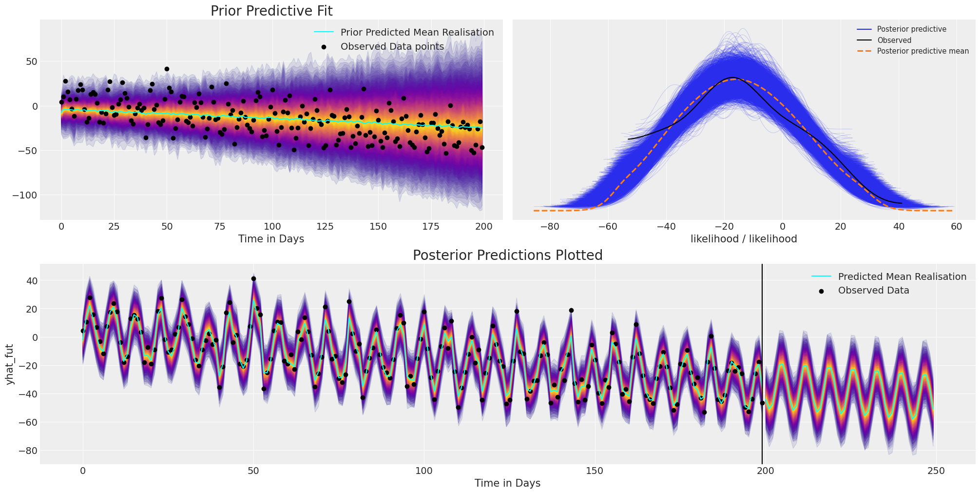
../_images/086ce40fad0e3bc0c9c718da0dfdb5a574c84aab65e5f6143f71fc0a52a227c7.png

我们可以在这里看到模型拟合如何再次恢复数据的广泛结构和趋势，但此外，我们还捕获了季节性效应的振荡并将其投影到未来。

结束语#

贝叶斯模型的优势在很大程度上在于它为每个建模任务提供的灵活性。希望本笔记本让您了解在构建适合您用例的模型时值得考虑的各种组合。我们已经了解了贝叶斯结构时间序列预测方法如何揭示我们数据的潜在结构，并用于将该结构向前投影。我们已经了解了如何在数据生成模型中编码不同的假设，并使用后验预测检查来校准我们的模型以适应观测数据。

值得注意的是，在自回归建模的情况下，我们明确依赖于结构组件的学习后验分布。在这方面，我们认为以上是贝叶斯学习的一种纯粹（整洁地包含）的示例。

作者#

改编自 Nathaniel Forde 于 2022 年 10 月在 Examined Algorithms Blog 上的文章，作者为 Nathaniel Forde。

水印#

%load_ext watermark
%watermark -n -u -v -iv -w -p pytensor,aeppl,xarray

Last updated: Wed Nov 09 2022

Python implementation: CPython
Python version       : 3.9.0
IPython version      : 8.4.0

pytensor: 2.8.7
aeppl : 0.0.38
xarray: 2022.10.0

arviz     : 0.12.1
pymc      : 4.2.2
numpy     : 1.23.4
pandas    : 1.5.1
sys       : 3.9.0 (default, Nov 15 2020, 06:25:35) 
[Clang 10.0.0 ]
matplotlib: 3.6.1

Watermark: 2.3.1

许可声明#

本示例 галерея 中的所有笔记本均根据 MIT 许可证提供，该许可证允许修改和再分发用于任何用途，前提是保留版权和许可声明。

引用 PyMC 示例#

要引用此笔记本，请使用 Zenodo 为 pymc-examples 存储库提供的 DOI。

重要提示

许多笔记本改编自其他来源：博客、书籍……在这种情况下，您也应该引用原始来源。

另请记住引用您的代码使用的相关库。

这是一个 BibTeX 中的引用模板

@incollection{citekey,
  author    = "<notebook authors, see above>",
  title     = "<notebook title>",
  editor    = "PyMC Team",
  booktitle = "PyMC examples",
  doi       = "10.5281/zenodo.5654871"
}

一旦渲染后可能看起来像

分类

标签

使用结构自回归时间序列进行预测#

生成伪自回归数据#

指定模型#

预测步骤#

检查模型拟合和预测#

使情况复杂化#

将我们的模型包装成函数#

指定趋势模型#

进一步使情况复杂化#

指定趋势 + 季节性模型#

结束语#

作者#

水印#

许可声明#

引用 PyMC 示例#