贝叶斯向量自回归模型#

import os

import arviz as az
import matplotlib.pyplot as plt
import numpy as np
import pandas as pd
import pymc as pm
import statsmodels.api as sm

from pymc.sampling_jax import sample_blackjax_nuts

/Users/nathanielforde/mambaforge/envs/myjlabenv/lib/python3.11/site-packages/pymc/sampling/jax.py:39: UserWarning: This module is experimental.
  warnings.warn("This module is experimental.")

RANDOM_SEED = 8927
rng = np.random.default_rng(RANDOM_SEED)
az.style.use("arviz-darkgrid")
%config InlineBackend.figure_format = 'retina'

V(ector)A(uto)R(egression) 模型#

在本笔记本中，我们将概述贝叶斯向量自回归模型的应用。我们将借鉴 PYMC Labs 博客文章中的工作（参见 Vieira [无日期]）。这将是一个分为三个部分系列。在第一部分中，我们想展示如何在 PYMC 中拟合贝叶斯 VAR 模型。在第二部分中，我们将展示如何从拟合模型中提取额外的见解，通过脉冲响应分析，并从拟合的 VAR 模型中进行预测。在第三部分也是最后一部分中，我们将更详细地展示使用贝叶斯 VAR 模型的分层先验的好处。具体来说，我们将概述如何以及为什么实际上存在一系列精心制定的行业标准先验，这些先验适用于贝叶斯 VAR 建模。

在这篇文章中，我们将 (i) 在虚假数据上演示简单 VAR 模型的基本模式，并展示模型如何恢复真实数据生成参数，以及 (ii) 我们将展示一个应用于宏观经济数据的示例，并将结果与使用 statsmodels MLE 拟合在相同数据上实现的结果进行比较，以及 (iii) 展示一个估计多个国家的层次贝叶斯 VAR 模型的示例。

通用自回归模型#

简单自回归模型的思想是捕捉时间序列的过去观测值如何预测当前观测值的方式。因此，按照传统方式，如果我们将此建模为线性现象，我们将得到简单的自回归模型，其中当前值由过去值的加权线性组合和误差项预测。

\[ y_t = \alpha + \beta_{y0} \cdot y_{t-1} + \beta_{y1} \cdot y_{t-2} ... + \epsilon \]

对于预测当前观测值所需的滞后阶数。

VAR 模型是这种框架的一种泛化，因为它保留了线性组合方法，但允许我们一次对多个时间序列进行建模。因此，具体而言，这意味着 \(\mathbf{y}_{t}\) 是一个向量，其中

\[ \mathbf{y}_{T} = \nu + A_{1}\mathbf{y}_{T-1} + A_{2}\mathbf{y}_{T-2} ... A_{p}\mathbf{y}_{T-p} + \mathbf{e}_{t} \]

其中 As 是系数矩阵，用于与每个单独时间序列的过去值组合。例如，考虑一个经济学示例，其中我们旨在对每个变量对自身和他人的关系和相互影响进行建模。

\[\begin{split} \begin{bmatrix} gdp \\ inv \\ con \end{bmatrix}_{T} = \nu + A_{1}\begin{bmatrix} gdp \\ inv \\ con \end{bmatrix}_{T-1} + A_{2}\begin{bmatrix} gdp \\ inv \\ con \end{bmatrix}_{T-2} ... A_{p}\begin{bmatrix} gdp \\ inv \\ con \end{bmatrix}_{T-p} + \mathbf{e}_{t} \end{split}\]

这种结构是使用矩阵符号的紧凑表示。当我们拟合 VAR 模型时，我们试图估计的是确定最适合我们时间序列数据的线性组合性质的 A 矩阵。这种时间序列模型可以具有自回归或移动平均表示，并且细节对于 VAR 模型拟合的一些含义很重要。

我们将在本系列的下一个笔记本中看到，VAR 的移动平均表示如何使其自身适用于将模型中的协方差结构解释为表示组件时间序列之间的一种脉冲响应关系。

具有两个滞后项的具体规范#

矩阵符号对于建议模型的广泛模式很方便，但查看简单情况下的代数很有用。考虑将爱尔兰的 GDP 和消费描述为

\[ gdp_{t} = \beta_{gdp1} \cdot gdp_{t-1} + \beta_{gdp2} \cdot gdp_{t-2} + \beta_{cons1} \cdot cons_{t-1} + \beta_{cons2} \cdot cons_{t-2} + \epsilon_{gdp}\]

\[ cons_{t} = \beta_{cons1} \cdot cons_{t-1} + \beta_{cons2} \cdot cons_{t-2} + \beta_{gdp1} \cdot gdp_{t-1} + \beta_{gdp2} \cdot gdp_{t-2} + \epsilon_{cons}\]

通过这种方式，我们可以看到，如果我们能够估计 \(\beta\) 项，我们就得到了每个变量对另一个变量的双向影响的估计。这是建模的一个有用特征。在接下来的内容中，我应该强调我不是经济学家，我的目标只是展示这些模型的功能，而不是给你关于决定爱尔兰 GDP 数字的经济关系的决定性意见。

创建一些虚假数据#

def simulate_var(
    intercepts, coefs_yy, coefs_xy, coefs_xx, coefs_yx, noises=(1, 1), *, warmup=100, steps=200
):
    draws_y = np.zeros(warmup + steps)
    draws_x = np.zeros(warmup + steps)
    draws_y[:2] = intercepts[0]
    draws_x[:2] = intercepts[1]
    for step in range(2, warmup + steps):
        draws_y[step] = (
            intercepts[0]
            + coefs_yy[0] * draws_y[step - 1]
            + coefs_yy[1] * draws_y[step - 2]
            + coefs_xy[0] * draws_x[step - 1]
            + coefs_xy[1] * draws_x[step - 2]
            + rng.normal(0, noises[0])
        )
        draws_x[step] = (
            intercepts[1]
            + coefs_xx[0] * draws_x[step - 1]
            + coefs_xx[1] * draws_x[step - 2]
            + coefs_yx[0] * draws_y[step - 1]
            + coefs_yx[1] * draws_y[step - 2]
            + rng.normal(0, noises[1])
        )
    return draws_y[warmup:], draws_x[warmup:]

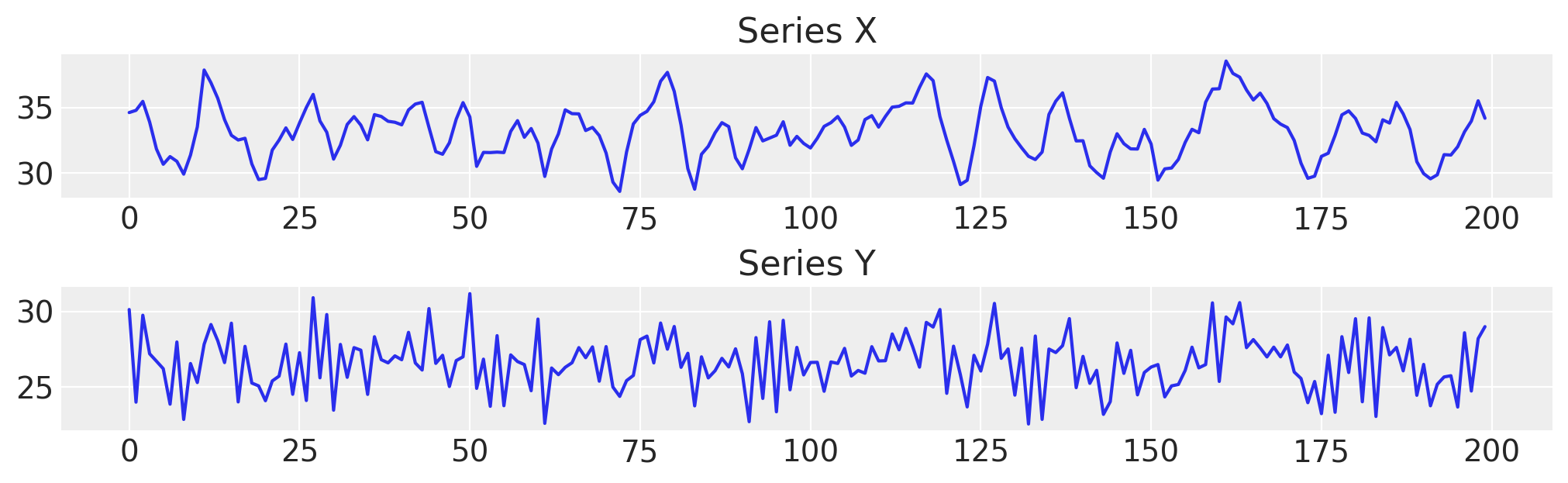
首先，我们生成一些具有已知参数的虚假数据。

var_y, var_x = simulate_var(
    intercepts=(18, 8),
    coefs_yy=(-0.8, 0),
    coefs_xy=(0.9, 0),
    coefs_xx=(1.3, -0.7),
    coefs_yx=(-0.1, 0.3),
)

df = pd.DataFrame({"x": var_x, "y": var_y})
df.head()

	x	y
0	34.606613	30.117581
1	34.773803	23.996700
2	35.455237	29.738941
3	33.886706	27.193417
4	31.837465	26.704728

fig, axs = plt.subplots(2, 1, figsize=(10, 3))
axs[0].plot(df["x"], label="x")
axs[0].set_title("Series X")
axs[1].plot(df["y"], label="y")
axs[1].set_title("Series Y");

../_images/ecc3bd5333e15cb66600373124e070d5a3e3bc9eeaf273614597721ef6ea9aa9.png

处理多个滞后和不同维度#

当对多个时间序列进行建模并考虑可能需要在模型中包含的任意数量的滞后时，我们需要将一些模型定义抽象到辅助函数中。一个例子将使这一点更清楚一些。

### Define a helper function that will construct our autoregressive step for the marginal contribution of each lagged
### term in each of the respective time series equations
def calc_ar_step(lag_coefs, n_eqs, n_lags, df):
    ars = []
    for j in range(n_eqs):
        ar = pm.math.sum(
            [
                pm.math.sum(lag_coefs[j, i] * df.values[n_lags - (i + 1) : -(i + 1)], axis=-1)
                for i in range(n_lags)
            ],
            axis=0,
        )
        ars.append(ar)
    beta = pm.math.stack(ars, axis=-1)

    return beta


### Make the model in such a way that it can handle different specifications of the likelihood term
### and can be run for simple prior predictive checks. This latter functionality is important for debugging of
### shape handling issues. Building a VAR model involves quite a few moving parts and it is handy to
### inspect the shape implied in the prior predictive checks.
def make_model(n_lags, n_eqs, df, priors, mv_norm=True, prior_checks=True):
    coords = {
        "lags": np.arange(n_lags) + 1,
        "equations": df.columns.tolist(),
        "cross_vars": df.columns.tolist(),
        "time": [x for x in df.index[n_lags:]],
    }

    with pm.Model(coords=coords) as model:
        lag_coefs = pm.Normal(
            "lag_coefs",
            mu=priors["lag_coefs"]["mu"],
            sigma=priors["lag_coefs"]["sigma"],
            dims=["equations", "lags", "cross_vars"],
        )
        alpha = pm.Normal(
            "alpha", mu=priors["alpha"]["mu"], sigma=priors["alpha"]["sigma"], dims=("equations",)
        )
        data_obs = pm.Data("data_obs", df.values[n_lags:], dims=["time", "equations"], mutable=True)

        betaX = calc_ar_step(lag_coefs, n_eqs, n_lags, df)
        betaX = pm.Deterministic(
            "betaX",
            betaX,
            dims=[
                "time",
            ],
        )
        mean = alpha + betaX

        if mv_norm:
            n = df.shape[1]
            ## Under the hood the LKJ prior will retain the correlation matrix too.
            noise_chol, _, _ = pm.LKJCholeskyCov(
                "noise_chol",
                eta=priors["noise_chol"]["eta"],
                n=n,
                sd_dist=pm.HalfNormal.dist(sigma=priors["noise_chol"]["sigma"]),
            )
            obs = pm.MvNormal(
                "obs", mu=mean, chol=noise_chol, observed=data_obs, dims=["time", "equations"]
            )
        else:
            ## This is an alternative likelihood that can recover sensible estimates of the coefficients
            ## But lacks the multivariate correlation between the timeseries.
            sigma = pm.HalfNormal("noise", sigma=priors["noise"]["sigma"], dims=["equations"])
            obs = pm.Normal(
                "obs", mu=mean, sigma=sigma, observed=data_obs, dims=["time", "equations"]
            )

        if prior_checks:
            idata = pm.sample_prior_predictive()
            return model, idata
        else:
            idata = pm.sample_prior_predictive()
            idata.extend(pm.sample(draws=2000, random_seed=130))
            pm.sample_posterior_predictive(idata, extend_inferencedata=True, random_seed=rng)
    return model, idata

该模型在自回归计算中具有确定性成分，这是每个时间步都需要的，但这里的关键点是我们将 VAR 的似然性建模为具有特定协方差关系的多元正态分布。这些协方差关系的估计给出了关于我们的组件时间序列彼此相关的方式的主要见解。

我们将检查具有 2 个滞后和 2 个方程的 VAR 的结构

n_lags = 2
n_eqs = 2
priors = {
    "lag_coefs": {"mu": 0.3, "sigma": 1},
    "alpha": {"mu": 15, "sigma": 5},
    "noise_chol": {"eta": 1, "sigma": 1},
    "noise": {"sigma": 1},
}

model, idata = make_model(n_lags, n_eqs, df, priors)
pm.model_to_graphviz(model)

Sampling: [alpha, lag_coefs, noise_chol, obs]

../_images/46db3979a328b9ac4ca045fdf34c75b2eb372ec81c2aa8d06daddab5b61b7c29.svg

另一个具有 3 个滞后和 2 个方程的 VAR。

n_lags = 3
n_eqs = 2
model, idata = make_model(n_lags, n_eqs, df, priors)
for rv, shape in model.eval_rv_shapes().items():
    print(f"{rv:>11}: shape={shape}")
pm.model_to_graphviz(model)

Sampling: [alpha, lag_coefs, noise_chol, obs]

  lag_coefs: shape=(2, 3, 2)
      alpha: shape=(2,)
noise_chol_cholesky-cov-packed__: shape=(3,)
 noise_chol: shape=(3,)

../_images/b0e658b7e9bee038b23b6d2680e8c0554015e9c3dce1186a5f8db9caf47ea709.svg

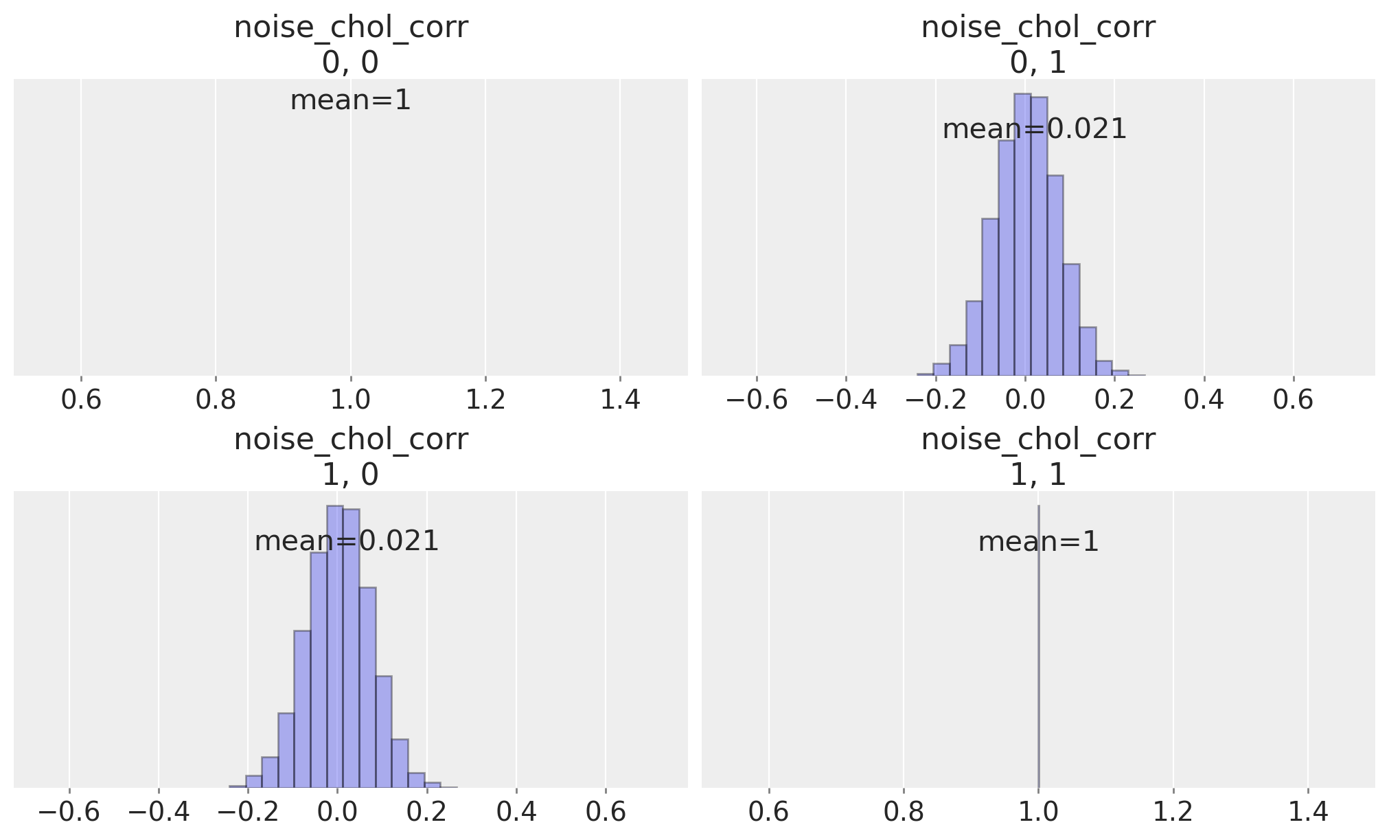
我们可以检查时间序列之间的相关矩阵，该矩阵由先验规范暗示，以查看我们是否允许了它们相关性的平坦均匀先验。

ax = az.plot_posterior(
    idata,
    var_names="noise_chol_corr",
    hdi_prob="hide",
    group="prior",
    point_estimate="mean",
    grid=(2, 2),
    kind="hist",
    ec="black",
    figsize=(10, 4),
)

../_images/30e5645b049e2276555bfba26d9640e5499c83d2824f9614e964ddf5c6f2b6cf.png

现在我们将拟合具有 2 个滞后和 2 个方程的 VAR

n_lags = 2
n_eqs = 2
model, idata_fake_data = make_model(n_lags, n_eqs, df, priors, prior_checks=False)

Sampling: [alpha, lag_coefs, noise_chol, obs]
Auto-assigning NUTS sampler...
Initializing NUTS using jitter+adapt_diag...
Multiprocess sampling (4 chains in 4 jobs)
NUTS: [lag_coefs, alpha, noise_chol]

100.00% [12000/12000 05:59<00:00 采样 4 条链, 0 个发散]

Sampling 4 chains for 1_000 tune and 2_000 draw iterations (4_000 + 8_000 draws total) took 360 seconds.
Sampling: [obs]

100.00% [8000/8000 02:11<00:00]

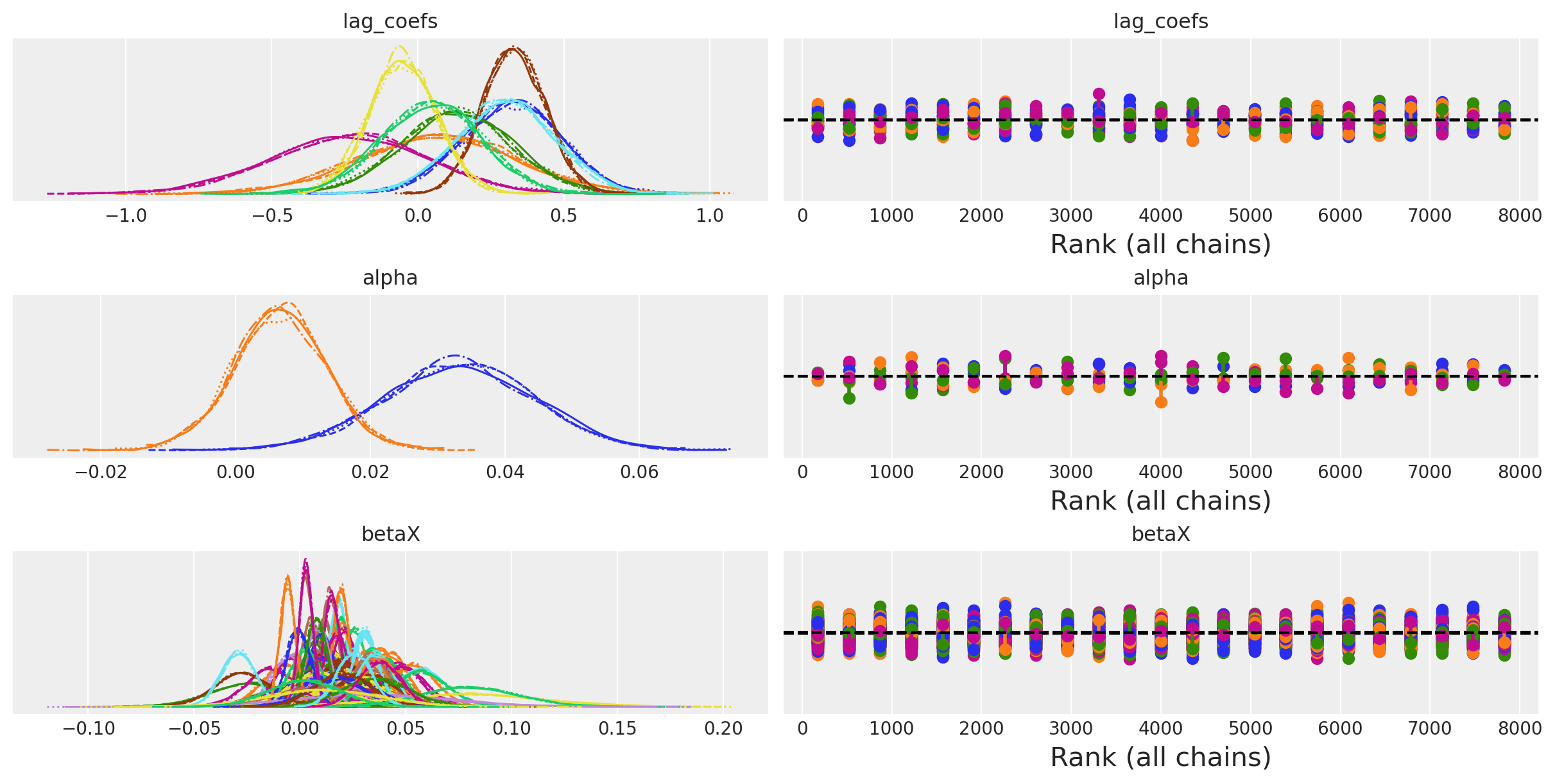
我们现在将绘制一些结果，以查看参数是否被大致恢复。alpha 参数匹配良好，但各个滞后系数显示出差异。

az.summary(idata_fake_data, var_names=["alpha", "lag_coefs", "noise_chol_corr"])

/Users/nathanielforde/mambaforge/envs/myjlabenv/lib/python3.11/site-packages/arviz/stats/diagnostics.py:584: RuntimeWarning: invalid value encountered in scalar divide
  (between_chain_variance / within_chain_variance + num_samples - 1) / (num_samples)

	均值	标准差	hdi_3%	hdi_97%	mcse_mean	mcse_sd	ess_bulk	ess_tail	r_hat
alpha[x]	8.607	1.765	5.380	12.076	0.029	0.020	3823.0	4602.0	1.0
alpha[y]	17.094	1.778	13.750	20.431	0.027	0.019	4188.0	5182.0	1.0
lag_coefs[x, 1, x]	1.333	0.062	1.218	1.450	0.001	0.001	5564.0	4850.0	1.0
lag_coefs[x, 1, y]	-0.120	0.069	-0.247	0.011	0.001	0.001	3739.0	4503.0	1.0
lag_coefs[x, 2, x]	-0.711	0.097	-0.890	-0.527	0.002	0.001	3629.0	4312.0	1.0
lag_coefs[x, 2, y]	0.267	0.073	0.126	0.403	0.001	0.001	3408.0	4318.0	1.0
lag_coefs[y, 1, x]	0.838	0.061	0.718	0.948	0.001	0.001	5203.0	5345.0	1.0
lag_coefs[y, 1, y]	-0.800	0.069	-0.932	-0.673	0.001	0.001	3749.0	5131.0	1.0
lag_coefs[y, 2, x]	0.094	0.097	-0.087	0.277	0.002	0.001	3573.0	4564.0	1.0
lag_coefs[y, 2, y]	-0.004	0.074	-0.145	0.133	0.001	0.001	3448.0	4484.0	1.0
noise_chol_corr[0, 0]	1.000	0.000	1.000	1.000	0.000	0.000	8000.0	8000.0	NaN
noise_chol_corr[0, 1]	0.021	0.072	-0.118	0.152	0.001	0.001	6826.0	5061.0	1.0
noise_chol_corr[1, 0]	0.021	0.072	-0.118	0.152	0.001	0.001	6826.0	5061.0	1.0
noise_chol_corr[1, 1]	1.000	0.000	1.000	1.000	0.000	0.000	7813.0	7824.0	1.0

az.plot_posterior(idata_fake_data, var_names=["alpha"], ref_val=[8, 18]);

../_images/4d7eb64f5ff15a8229c61d0b7226c784c23a4180382b2c37079f45a01dbfe5c0.png

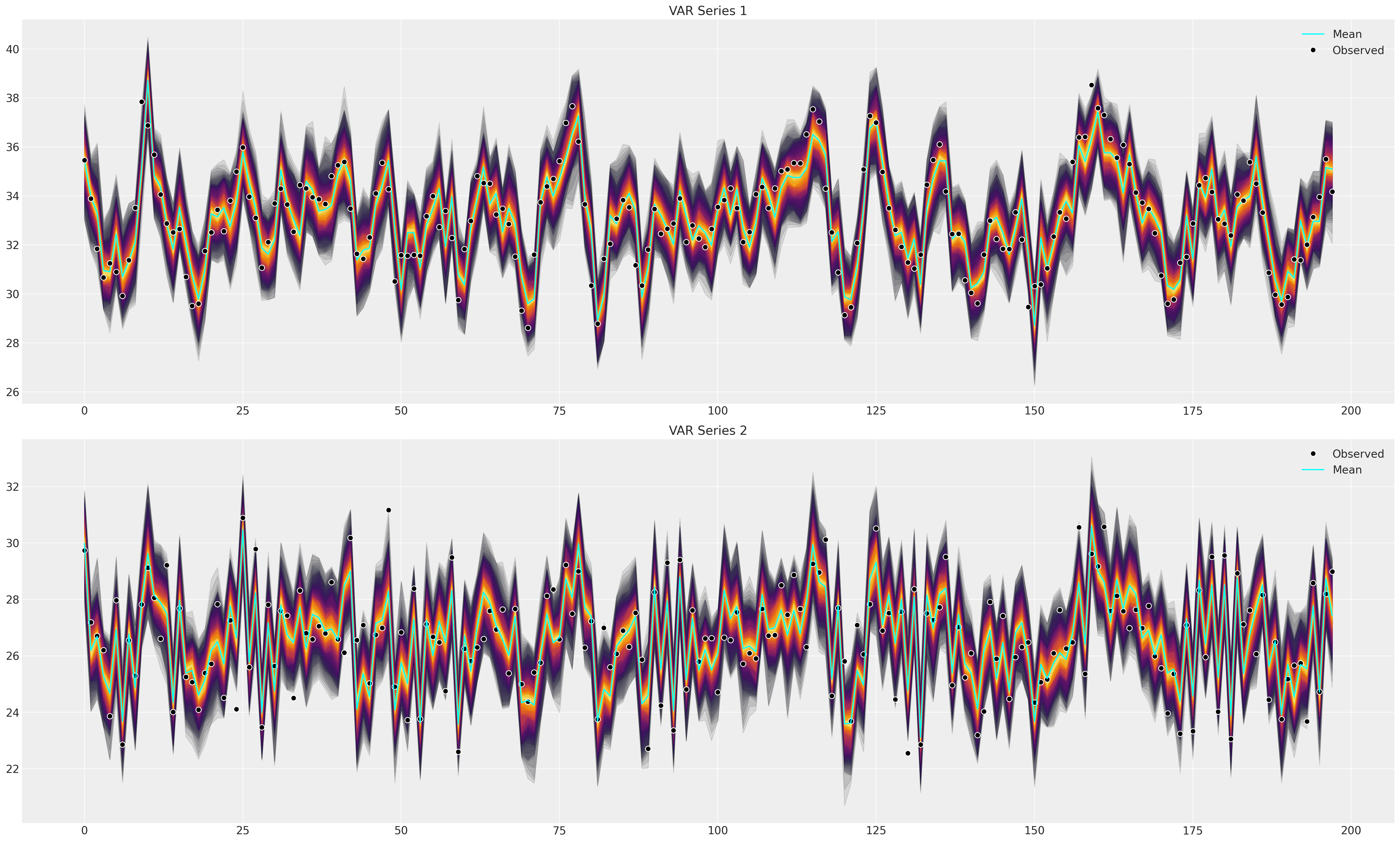
接下来，我们将绘制后验预测分布，以检查拟合模型是否可以捕捉到观测数据中的模式。这是拟合优度的主要测试。

def shade_background(ppc, ax, idx, palette="cividis"):
    palette = palette
    cmap = plt.get_cmap(palette)
    percs = np.linspace(51, 99, 100)
    colors = (percs - np.min(percs)) / (np.max(percs) - np.min(percs))
    for i, p in enumerate(percs[::-1]):
        upper = np.percentile(
            ppc[:, idx, :],
            p,
            axis=1,
        )
        lower = np.percentile(
            ppc[:, idx, :],
            100 - p,
            axis=1,
        )
        color_val = colors[i]
        ax[idx].fill_between(
            x=np.arange(ppc.shape[0]),
            y1=upper.flatten(),
            y2=lower.flatten(),
            color=cmap(color_val),
            alpha=0.1,
        )


def plot_ppc(idata, df, group="posterior_predictive"):
    fig, axs = plt.subplots(2, 1, figsize=(25, 15))
    df = pd.DataFrame(idata_fake_data["observed_data"]["obs"].data, columns=["x", "y"])
    axs = axs.flatten()
    ppc = az.extract(idata, group=group, num_samples=100)["obs"]
    # Minus the lagged terms and the constant
    shade_background(ppc, axs, 0, "inferno")
    axs[0].plot(np.arange(ppc.shape[0]), ppc[:, 0, :].mean(axis=1), color="cyan", label="Mean")
    axs[0].plot(df["x"], "o", mfc="black", mec="white", mew=1, markersize=7, label="Observed")
    axs[0].set_title("VAR Series 1")
    axs[0].legend()
    shade_background(ppc, axs, 1, "inferno")
    axs[1].plot(df["y"], "o", mfc="black", mec="white", mew=1, markersize=7, label="Observed")
    axs[1].plot(np.arange(ppc.shape[0]), ppc[:, 1, :].mean(axis=1), color="cyan", label="Mean")
    axs[1].set_title("VAR Series 2")
    axs[1].legend()


plot_ppc(idata_fake_data, df)

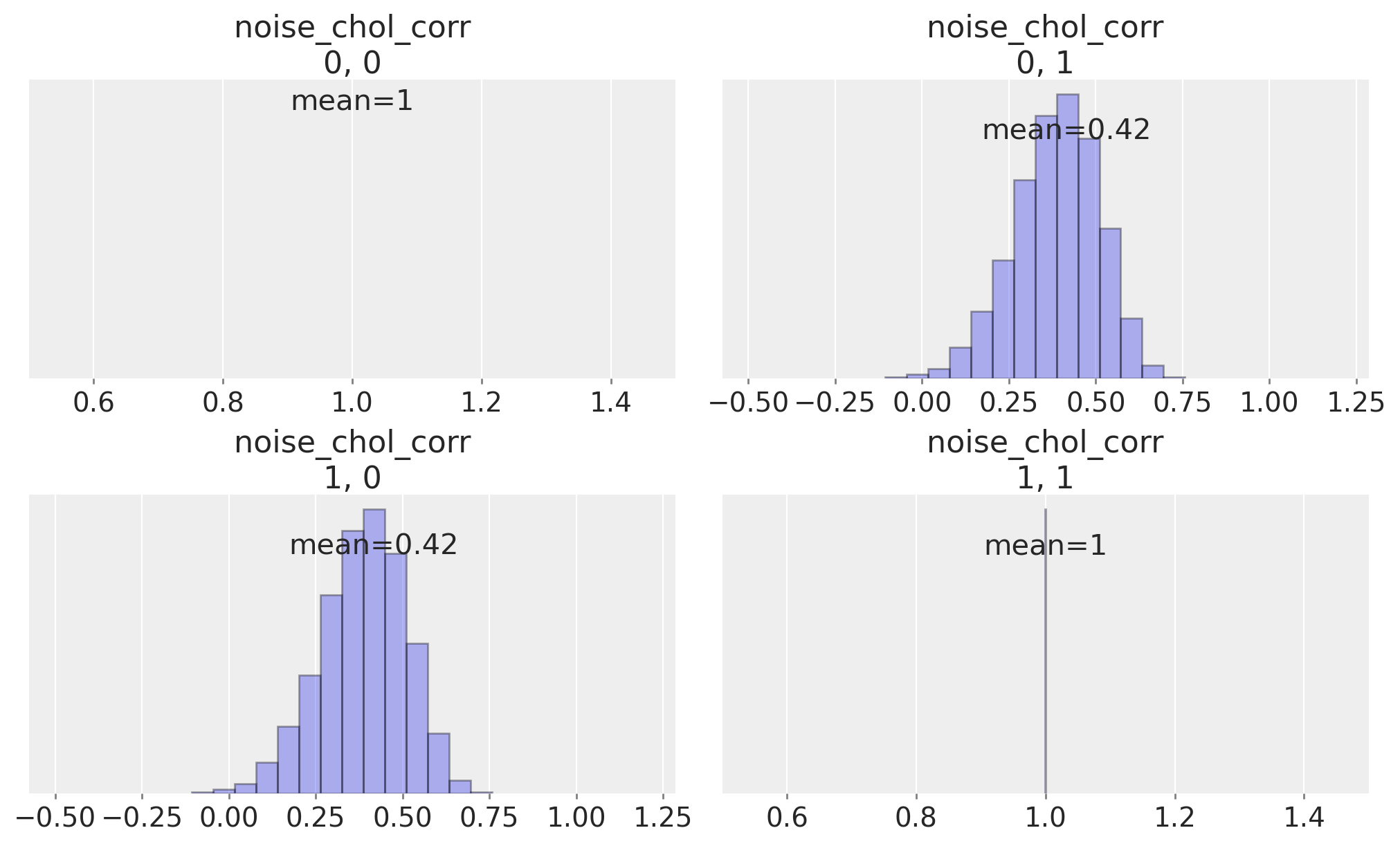
../_images/4cc2d4d22fd292017c1b8597b2f9e23929a0a13ed2936b03e14f9038c40ccd84.png

再次，我们可以检查相关参数的学习后验分布。

ax = az.plot_posterior(
    idata_fake_data,
    var_names="noise_chol_corr",
    hdi_prob="hide",
    point_estimate="mean",
    grid=(2, 2),
    kind="hist",
    ec="black",
    figsize=(10, 6),
)

../_images/4ba85f65960464ed574fbf89fe8162e4faade29acef50963c3c62b6cd7d49f0d.png

应用理论：宏观经济时间序列#

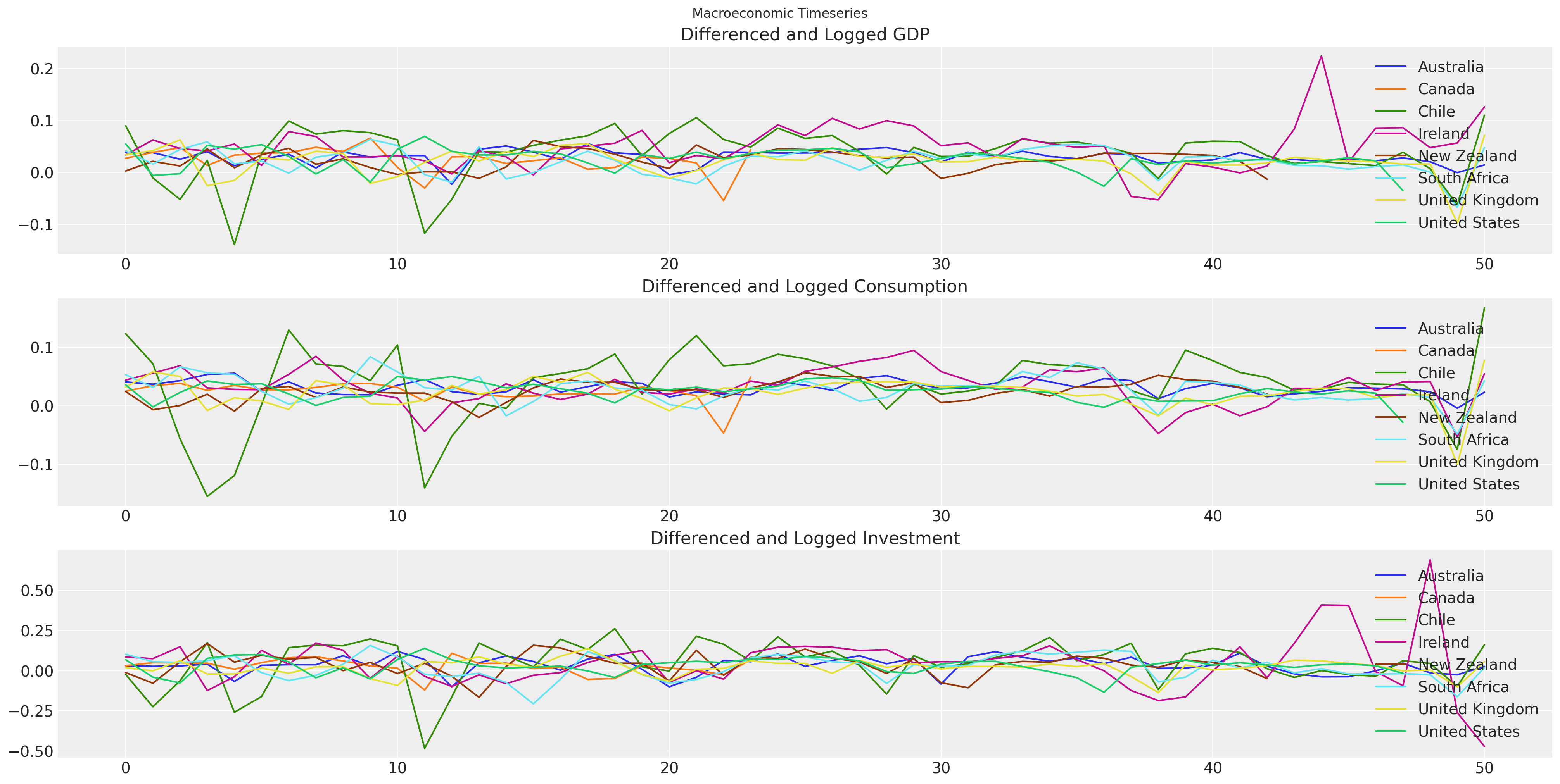
数据来自世界银行的世界发展指标。特别是，我们正在提取 1970 年以来所有国家的 GDP、消费和固定资本形成总额（投资）的年度值。时间序列模型通常在整个序列中具有稳定的均值时效果最佳，因此对于估计过程，我们采用了这些序列的一阶差分和自然对数。

try:
    gdp_hierarchical = pd.read_csv(
        os.path.join("..", "data", "gdp_data_hierarchical_clean.csv"), index_col=0
    )
except FileNotFoundError:
    gdp_hierarchical = pd.read_csv(pm.get_data("gdp_data_hierarchical_clean.csv"), ...)

gdp_hierarchical

	国家	iso2c	iso3c	年份	GDP	CONS	GFCF	dl_gdp	dl_cons	dl_gfcf	more_than_10	时间
1	澳大利亚	AU	AUS	1971	4.647670e+11	3.113170e+11	7.985100e+10	0.039217	0.040606	0.031705	True	1
2	澳大利亚	AU	AUS	1972	4.829350e+11	3.229650e+11	8.209200e+10	0.038346	0.036732	0.027678	True	2
3	澳大利亚	AU	AUS	1973	4.955840e+11	3.371070e+11	8.460300e+10	0.025855	0.042856	0.030129	True	3
4	澳大利亚	AU	AUS	1974	5.159300e+11	3.556010e+11	8.821400e+10	0.040234	0.053409	0.041796	True	4
5	澳大利亚	AU	AUS	1975	5.228210e+11	3.759000e+11	8.255900e+10	0.013268	0.055514	-0.066252	True	5
...	...	...	...	...	...	...	...	...	...	...	...	...
366	美国	US	USA	2016	1.850960e+13	1.522497e+13	3.802207e+12	0.016537	0.023425	0.021058	True	44
367	美国	US	USA	2017	1.892712e+13	1.553075e+13	3.947418e+12	0.022306	0.019885	0.037480	True	45
368	美国	US	USA	2018	1.947957e+13	1.593427e+13	4.119951e+12	0.028771	0.025650	0.042780	True	46
369	美国	US	USA	2019	1.992544e+13	1.627888e+13	4.248643e+12	0.022631	0.021396	0.030758	True	47
370	美国	US	USA	2020	1.924706e+13	1.582501e+13	4.182801e+12	-0.034639	-0.028277	-0.015619	True	48

370 行 × 12 列

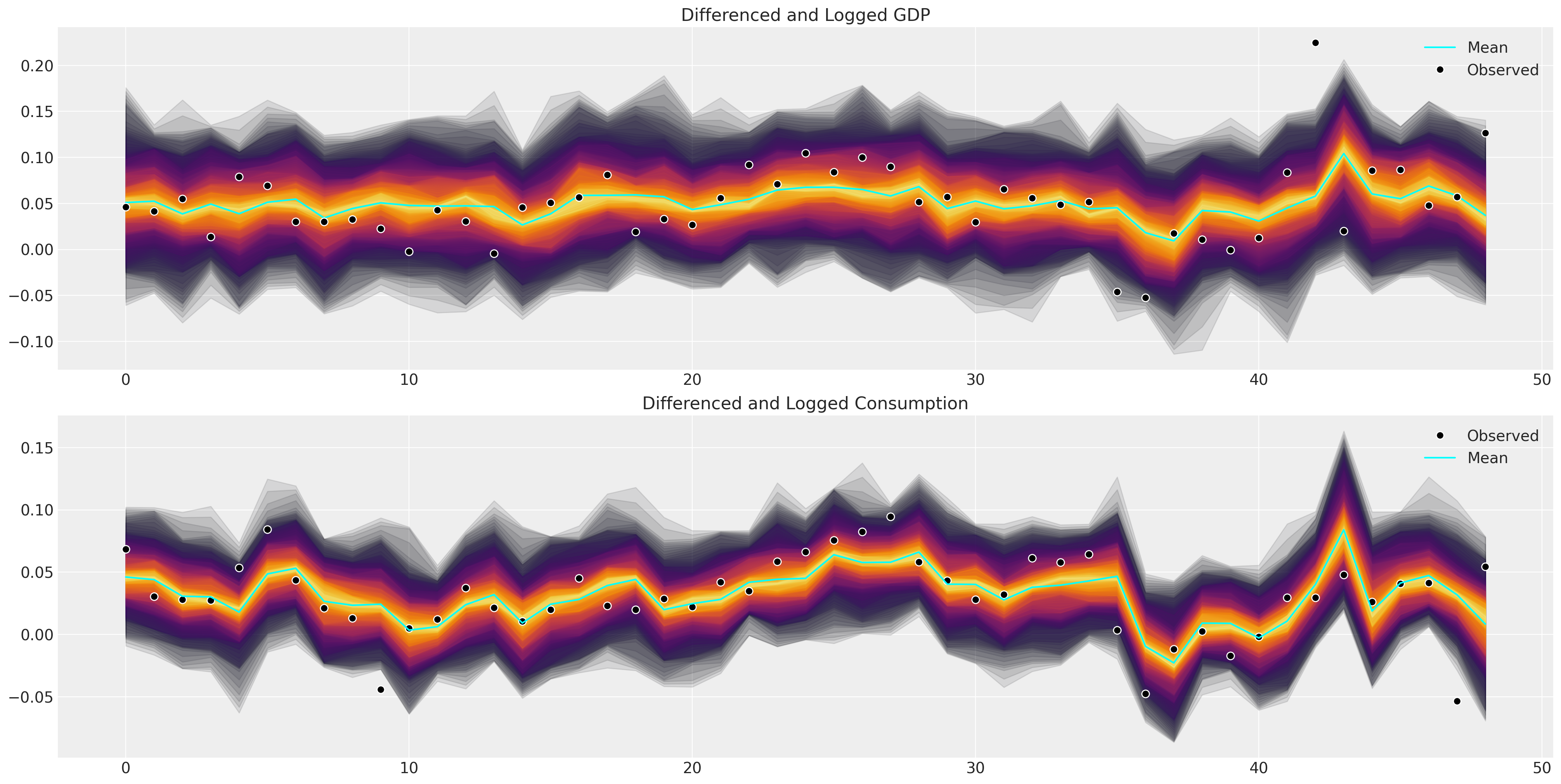
fig, axs = plt.subplots(3, 1, figsize=(20, 10))
for country in gdp_hierarchical["country"].unique():
    temp = gdp_hierarchical[gdp_hierarchical["country"] == country].reset_index()
    axs[0].plot(temp["dl_gdp"], label=f"{country}")
    axs[1].plot(temp["dl_cons"], label=f"{country}")
    axs[2].plot(temp["dl_gfcf"], label=f"{country}")
axs[0].set_title("Differenced and Logged GDP")
axs[1].set_title("Differenced and Logged Consumption")
axs[2].set_title("Differenced and Logged Investment")
axs[0].legend()
axs[1].legend()
axs[2].legend()
plt.suptitle("Macroeconomic Timeseries");

../_images/4e2642a8e46e880c72e474b3db11d9728e98dc58908f61da9d28e92bee721052.png

爱尔兰的经济状况#

爱尔兰因其 GDP 数字而臭名昭著，这些数字在很大程度上是外国直接投资的产物，并且近年来由于向大型跨国公司提供的投资和税收协议而被夸大超出预期。我们将在此处仅关注 GDP 和消费之间的关系。我们只想展示 VAR 估计的机制，您不应过多解读随后的分析。

ireland_df = gdp_hierarchical[gdp_hierarchical["country"] == "Ireland"]
ireland_df.reset_index(inplace=True, drop=True)
ireland_df.head()

	国家	iso2c	iso3c	年份	GDP	CONS	GFCF	dl_gdp	dl_cons	dl_gfcf	more_than_10	时间
0	爱尔兰	IE	IRL	1971	3.314234e+10	2.897699e+10	8.317518e+09	0.034110	0.043898	0.085452	True	1
1	爱尔兰	IE	IRL	1972	3.529322e+10	3.063538e+10	8.967782e+09	0.062879	0.055654	0.075274	True	2
2	爱尔兰	IE	IRL	1973	3.695956e+10	3.280221e+10	1.041728e+10	0.046134	0.068340	0.149828	True	3
3	爱尔兰	IE	IRL	1974	3.853412e+10	3.381524e+10	9.207243e+09	0.041720	0.030416	-0.123476	True	4
4	爱尔兰	IE	IRL	1975	4.071386e+10	3.477232e+10	8.874887e+09	0.055024	0.027910	-0.036765	True	5

az.plot_trace(idata_ireland, var_names=["lag_coefs", "alpha", "betaX"], kind="rank_vlines");

../_images/063abe8a9272f0339cf7f3d814d8505c716f95d2846242b4017d6f23a605059b.png

def plot_ppc_macro(idata, df, group="posterior_predictive"):
    df = pd.DataFrame(idata["observed_data"]["obs"].data, columns=["dl_gdp", "dl_cons"])
    fig, axs = plt.subplots(2, 1, figsize=(20, 10))
    axs = axs.flatten()
    ppc = az.extract(idata, group=group, num_samples=100)["obs"]

    shade_background(ppc, axs, 0, "inferno")
    axs[0].plot(np.arange(ppc.shape[0]), ppc[:, 0, :].mean(axis=1), color="cyan", label="Mean")
    axs[0].plot(df["dl_gdp"], "o", mfc="black", mec="white", mew=1, markersize=7, label="Observed")
    axs[0].set_title("Differenced and Logged GDP")
    axs[0].legend()
    shade_background(ppc, axs, 1, "inferno")
    axs[1].plot(df["dl_cons"], "o", mfc="black", mec="white", mew=1, markersize=7, label="Observed")
    axs[1].plot(np.arange(ppc.shape[0]), ppc[:, 1, :].mean(axis=1), color="cyan", label="Mean")
    axs[1].set_title("Differenced and Logged Consumption")
    axs[1].legend()


plot_ppc_macro(idata_ireland, ireland_df)

../_images/762ce8a1ab002a935bc3005e61db46f73334a5676f781fd91760e1a592adb28a.png

ax = az.plot_posterior(
    idata_ireland,
    var_names="noise_chol_corr",
    hdi_prob="hide",
    point_estimate="mean",
    grid=(2, 2),
    kind="hist",
    ec="black",
    figsize=(10, 6),
)

../_images/85dc433748b1cabd042f50cbea09d5fe9ea6c7cce63f2aabc01fc4c56657f7ba.png

与 Statsmodels 的比较#

值得将这些模型拟合与 Statsmodels 实现的模型拟合进行比较，只是为了看看我们是否可以恢复类似的故事。

VAR_model = sm.tsa.VAR(ireland_df[["dl_gdp", "dl_cons"]])
results = VAR_model.fit(2, trend="c")

results.params

	dl_gdp	dl_cons
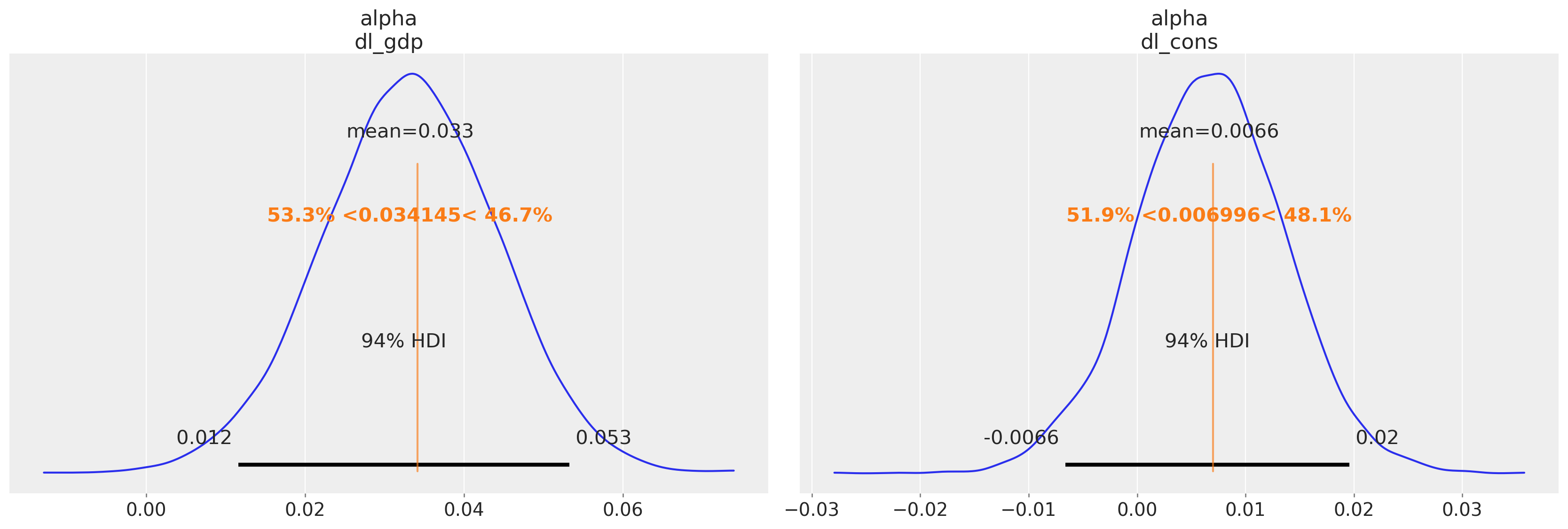
const	0.034145	0.006996
L1.dl_gdp	0.324904	0.330003
L1.dl_cons	0.076629	0.305824
L2.dl_gdp	0.137721	-0.053677
L2.dl_cons	-0.278745	0.033728

截距参数与我们的贝叶斯模型大致一致，但由滞后项的估计值定义的隐含关系存在一些差异。

corr = pd.DataFrame(results.resid_corr, columns=["dl_gdp", "dl_cons"])
corr.index = ["dl_gdp", "dl_cons"]
corr

	dl_gdp	dl_cons
dl_gdp	1.000000	0.435807
dl_cons	0.435807	1.000000

statsmodels 报告的残差相关性估计值与我们的贝叶斯模型中变量之间的多元高斯相关性非常吻合。

az.summary(idata_ireland, var_names=["alpha", "lag_coefs", "noise_chol_corr"])

/Users/nathanielforde/mambaforge/envs/myjlabenv/lib/python3.11/site-packages/arviz/stats/diagnostics.py:584: RuntimeWarning: invalid value encountered in scalar divide
  (between_chain_variance / within_chain_variance + num_samples - 1) / (num_samples)

	均值	标准差	hdi_3%	hdi_97%	mcse_mean	mcse_sd	ess_bulk	ess_tail	r_hat
alpha[dl_gdp]	0.033	0.011	0.012	0.053	0.000	0.000	6683.0	5919.0	1.0
alpha[dl_cons]	0.007	0.007	-0.007	0.020	0.000	0.000	7651.0	5999.0	1.0
lag_coefs[dl_gdp, 1, dl_gdp]	0.321	0.170	0.008	0.642	0.002	0.002	6984.0	6198.0	1.0
lag_coefs[dl_gdp, 1, dl_cons]	0.071	0.273	-0.447	0.582	0.003	0.003	7376.0	5466.0	1.0
lag_coefs[dl_gdp, 2, dl_gdp]	0.133	0.190	-0.228	0.488	0.002	0.002	7471.0	6128.0	1.0
lag_coefs[dl_gdp, 2, dl_cons]	-0.235	0.269	-0.748	0.259	0.003	0.002	8085.0	5963.0	1.0
lag_coefs[dl_cons, 1, dl_gdp]	0.331	0.106	0.133	0.528	0.001	0.001	7670.0	6360.0	1.0
lag_coefs[dl_cons, 1, dl_cons]	0.302	0.170	-0.012	0.616	0.002	0.001	7963.0	6150.0	1.0
lag_coefs[dl_cons, 2, dl_gdp]	-0.054	0.118	-0.279	0.163	0.001	0.001	8427.0	6296.0	1.0
lag_coefs[dl_cons, 2, dl_cons]	0.048	0.170	-0.259	0.378	0.002	0.002	8669.0	6264.0	1.0
noise_chol_corr[0, 0]	1.000	0.000	1.000	1.000	0.000	0.000	8000.0	8000.0	NaN
noise_chol_corr[0, 1]	0.416	0.123	0.180	0.633	0.001	0.001	9155.0	6052.0	1.0
noise_chol_corr[1, 0]	0.416	0.123	0.180	0.633	0.001	0.001	9155.0	6052.0	1.0
noise_chol_corr[1, 1]	1.000	0.000	1.000	1.000	0.000	0.000	7871.0	8000.0	1.0

我们绘制 alpha 参数估计值与 Statsmodels 估计值的对比图

az.plot_posterior(idata_ireland, var_names=["alpha"], ref_val=[0.034145, 0.006996]);

../_images/bca8db365b5899de2b68e81fd2f6816c9025404bf29b6a61a603314acfef7a33.png

az.plot_posterior(
    idata_ireland,
    var_names=["lag_coefs"],
    ref_val=[0.330003, -0.053677],
    coords={"equations": "dl_cons", "lags": [1, 2], "cross_vars": "dl_gdp"},
);

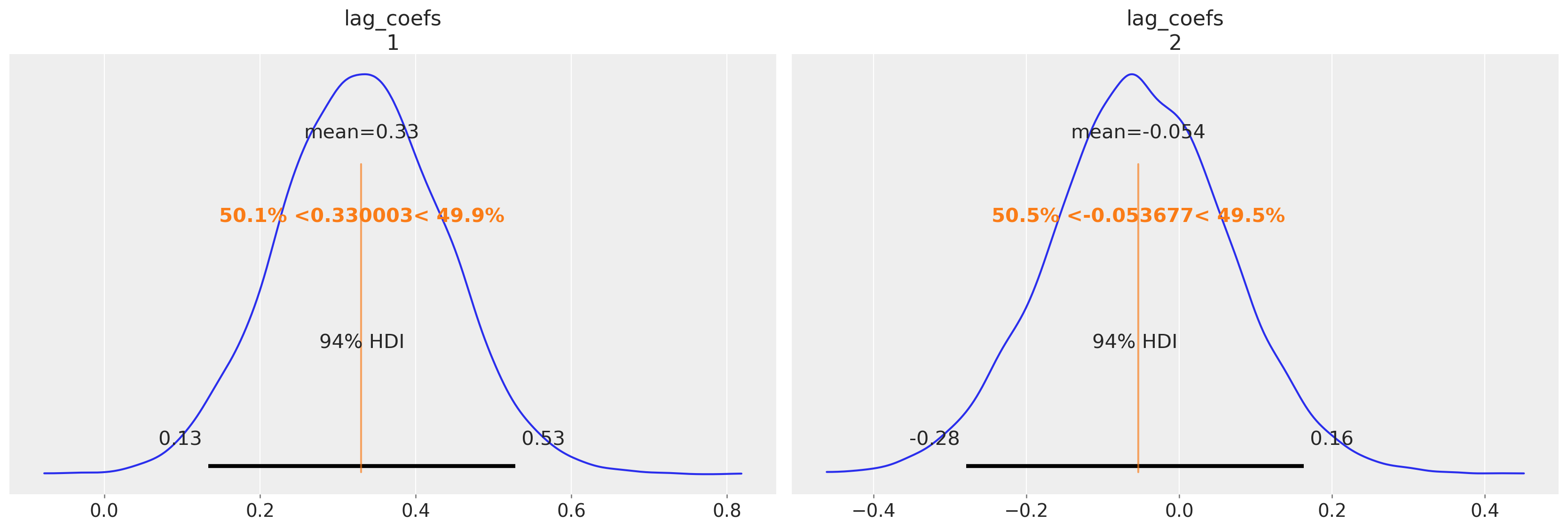
../_images/21fd827e56c649e0d9da4ecfc65752ccc706f5f52b2ef06a1ba352b67cd08968.png

我们再次可以看到贝叶斯 VAR 模型如何恢复许多相同的故事。两个方程的 alpha 项的估计值具有相似的量级，并且第一个滞后的 GDP 数字与消费之间存在明显的关系，以及非常相似的协方差结构。

添加贝叶斯扭曲：分层 VAR#

此外，如果我们想对多个国家以及国家层面这些经济指标之间的关系进行建模，我们可以添加一些分层参数。这在我们的时间序列数据相当短的情况下是一种有用的技术，因为它允许我们“借用”跨国家的信息来告知关键参数的估计。

def make_hierarchical_model(n_lags, n_eqs, df, group_field, prior_checks=True):
    cols = [col for col in df.columns if col != group_field]
    coords = {"lags": np.arange(n_lags) + 1, "equations": cols, "cross_vars": cols}

    groups = df[group_field].unique()

    with pm.Model(coords=coords) as model:
        ## Hierarchical Priors
        rho = pm.Beta("rho", alpha=2, beta=2)
        alpha_hat_location = pm.Normal("alpha_hat_location", 0, 0.1)
        alpha_hat_scale = pm.InverseGamma("alpha_hat_scale", 3, 0.5)
        beta_hat_location = pm.Normal("beta_hat_location", 0, 0.1)
        beta_hat_scale = pm.InverseGamma("beta_hat_scale", 3, 0.5)
        omega_global, _, _ = pm.LKJCholeskyCov(
            "omega_global", n=n_eqs, eta=1.0, sd_dist=pm.Exponential.dist(1)
        )

        for grp in groups:
            df_grp = df[df[group_field] == grp][cols]
            z_scale_beta = pm.InverseGamma(f"z_scale_beta_{grp}", 3, 0.5)
            z_scale_alpha = pm.InverseGamma(f"z_scale_alpha_{grp}", 3, 0.5)
            lag_coefs = pm.Normal(
                f"lag_coefs_{grp}",
                mu=beta_hat_location,
                sigma=beta_hat_scale * z_scale_beta,
                dims=["equations", "lags", "cross_vars"],
            )
            alpha = pm.Normal(
                f"alpha_{grp}",
                mu=alpha_hat_location,
                sigma=alpha_hat_scale * z_scale_alpha,
                dims=("equations",),
            )

            betaX = calc_ar_step(lag_coefs, n_eqs, n_lags, df_grp)
            betaX = pm.Deterministic(f"betaX_{grp}", betaX)
            mean = alpha + betaX

            n = df_grp.shape[1]
            noise_chol, _, _ = pm.LKJCholeskyCov(
                f"noise_chol_{grp}", eta=10, n=n, sd_dist=pm.Exponential.dist(1)
            )
            omega = pm.Deterministic(f"omega_{grp}", rho * omega_global + (1 - rho) * noise_chol)
            obs = pm.MvNormal(f"obs_{grp}", mu=mean, chol=omega, observed=df_grp.values[n_lags:])

        if prior_checks:
            idata = pm.sample_prior_predictive()
            return model, idata
        else:
            idata = pm.sample_prior_predictive()
            idata.extend(sample_blackjax_nuts(2000, random_seed=120))
            pm.sample_posterior_predictive(idata, extend_inferencedata=True)
    return model, idata

模型设计允许通过允许我们将特定国家的估计值从分层均值移开来非中心化关键似然的参数化，用于每个国家组成部分。这是通过 rho * omega_global + (1 - rho) * noise_chol 行完成的。参数 rho 确定每个国家的数据对经济变量之间协方差关系估计的贡献份额。类似的特定国家调整使用 z_alpha_scale 和 z_beta_scale 参数进行。

df_final = gdp_hierarchical[["country", "dl_gdp", "dl_cons", "dl_gfcf"]]
model_full_test, idata_full_test = make_hierarchical_model(
    2,
    3,
    df_final,
    "country",
    prior_checks=False,
)

Sampling: [alpha_Australia, alpha_Canada, alpha_Chile, alpha_Ireland, alpha_New Zealand, alpha_South Africa, alpha_United Kingdom, alpha_United States, alpha_hat_location, alpha_hat_scale, beta_hat_location, beta_hat_scale, lag_coefs_Australia, lag_coefs_Canada, lag_coefs_Chile, lag_coefs_Ireland, lag_coefs_New Zealand, lag_coefs_South Africa, lag_coefs_United Kingdom, lag_coefs_United States, noise_chol_Australia, noise_chol_Canada, noise_chol_Chile, noise_chol_Ireland, noise_chol_New Zealand, noise_chol_South Africa, noise_chol_United Kingdom, noise_chol_United States, obs_Australia, obs_Canada, obs_Chile, obs_Ireland, obs_New Zealand, obs_South Africa, obs_United Kingdom, obs_United States, omega_global, rho, z_scale_alpha_Australia, z_scale_alpha_Canada, z_scale_alpha_Chile, z_scale_alpha_Ireland, z_scale_alpha_New Zealand, z_scale_alpha_South Africa, z_scale_alpha_United Kingdom, z_scale_alpha_United States, z_scale_beta_Australia, z_scale_beta_Canada, z_scale_beta_Chile, z_scale_beta_Ireland, z_scale_beta_New Zealand, z_scale_beta_South Africa, z_scale_beta_United Kingdom, z_scale_beta_United States]

Compiling...
Compilation time =  0:00:12.203665
Sampling...
Sampling time =  0:01:13.331452
Transforming variables...
Transformation time =  0:00:13.215405

Sampling: [obs_Australia, obs_Canada, obs_Chile, obs_Ireland, obs_New Zealand, obs_South Africa, obs_United Kingdom, obs_United States]

100.00% [8000/8000 07:19<00:00]

az.plot_trace(
    idata_full_test,
    var_names=["rho", "alpha_hat_location", "beta_hat_location", "omega_global"],
    kind="rank_vlines",
);

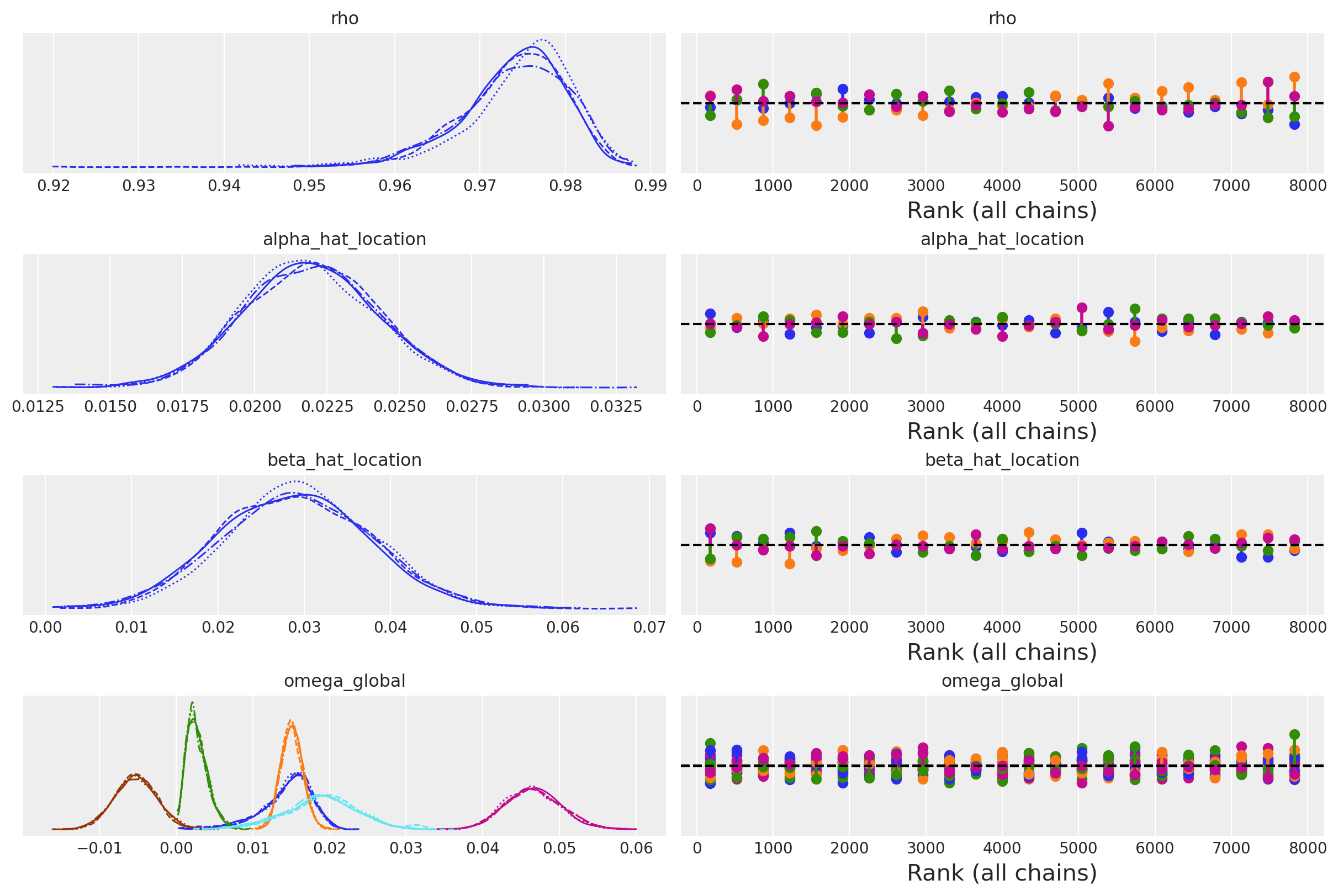
../_images/0973c34fb7f535c89c51d3f0de40d7b80c4c679fad12957b3cf064fb912b3160.png

接下来我们将看看一些汇总统计量，以及它们在不同国家之间的变化情况。

az.summary(
    idata_full_test,
    var_names=[
        "rho",
        "alpha_hat_location",
        "alpha_hat_scale",
        "beta_hat_location",
        "beta_hat_scale",
        "z_scale_alpha_Ireland",
        "z_scale_alpha_United States",
        "z_scale_beta_Ireland",
        "z_scale_beta_United States",
        "alpha_Ireland",
        "alpha_United States",
        "omega_global_corr",
        "lag_coefs_Ireland",
        "lag_coefs_United States",
    ],
)

/Users/nathanielforde/mambaforge/envs/myjlabenv/lib/python3.11/site-packages/arviz/stats/diagnostics.py:584: RuntimeWarning: invalid value encountered in scalar divide
  (between_chain_variance / within_chain_variance + num_samples - 1) / (num_samples)

	均值	标准差	hdi_3%	hdi_97%	mcse_mean	mcse_sd	ess_bulk	ess_tail	r_hat
rho	0.974	0.006	0.962	0.984	0.000	0.000	749.0	1354.0	1.00
alpha_hat_location	0.022	0.002	0.018	0.026	0.000	0.000	1642.0	3651.0	1.00
alpha_hat_scale	0.047	0.012	0.027	0.069	0.000	0.000	2933.0	1097.0	1.00
beta_hat_location	0.029	0.009	0.014	0.046	0.000	0.000	855.0	2218.0	1.00
beta_hat_scale	0.186	0.064	0.077	0.305	0.003	0.002	312.0	647.0	1.01
z_scale_alpha_Ireland	0.264	0.147	0.070	0.508	0.002	0.002	2074.0	854.0	1.00
z_scale_alpha_United States	0.132	0.066	0.045	0.245	0.001	0.001	8457.0	5680.0	1.00
z_scale_beta_Ireland	0.508	0.326	0.096	1.067	0.014	0.010	592.0	1294.0	1.00
z_scale_beta_United States	0.213	0.125	0.050	0.445	0.005	0.003	646.0	1423.0	1.00
alpha_Ireland[dl_gdp]	0.035	0.008	0.020	0.048	0.000	0.000	3446.0	4001.0	1.00
alpha_Ireland[dl_cons]	0.014	0.006	0.003	0.024	0.000	0.000	1597.0	4464.0	1.00
alpha_Ireland[dl_gfcf]	0.024	0.011	0.002	0.046	0.000	0.000	6768.0	5217.0	1.00
alpha_United States[dl_gdp]	0.021	0.003	0.015	0.026	0.000	0.000	2322.0	3773.0	1.00
alpha_United States[dl_cons]	0.020	0.003	0.015	0.025	0.000	0.000	2164.0	3321.0	1.00
alpha_United States[dl_gfcf]	0.024	0.005	0.015	0.034	0.000	0.000	4455.0	5176.0	1.00
omega_global_corr[0, 0]	1.000	0.000	1.000	1.000	0.000	0.000	8000.0	8000.0	NaN
omega_global_corr[0, 1]	0.980	0.019	0.944	1.000	0.000	0.000	2393.0	2273.0	1.00
omega_global_corr[0, 2]	0.916	0.033	0.854	0.977	0.001	0.001	915.0	763.0	1.00
omega_global_corr[1, 0]	0.980	0.019	0.944	1.000	0.000	0.000	2393.0	2273.0	1.00
omega_global_corr[1, 1]	1.000	0.000	1.000	1.000	0.000	0.000	7937.0	7898.0	1.00
omega_global_corr[1, 2]	0.879	0.045	0.794	0.960	0.001	0.001	1345.0	3018.0	1.00
omega_global_corr[2, 0]	0.916	0.033	0.854	0.977	0.001	0.001	915.0	763.0	1.00
omega_global_corr[2, 1]	0.879	0.045	0.794	0.960	0.001	0.001	1345.0	3018.0	1.00
omega_global_corr[2, 2]	1.000	0.000	1.000	1.000	0.000	0.000	8042.0	7890.0	1.00
lag_coefs_Ireland[dl_gdp, 1, dl_gdp]	0.012	0.080	-0.151	0.160	0.001	0.001	5559.0	3646.0	1.00
lag_coefs_Ireland[dl_gdp, 1, dl_cons]	0.007	0.086	-0.161	0.174	0.001	0.002	4661.0	3294.0	1.00
lag_coefs_Ireland[dl_gdp, 1, dl_gfcf]	0.057	0.037	-0.009	0.128	0.001	0.000	4699.0	4249.0	1.00
lag_coefs_Ireland[dl_gdp, 2, dl_gdp]	-0.005	0.087	-0.176	0.152	0.002	0.002	3099.0	2447.0	1.00
lag_coefs_Ireland[dl_gdp, 2, dl_cons]	0.003	0.088	-0.171	0.171	0.001	0.001	4239.0	2997.0	1.00
lag_coefs_Ireland[dl_gdp, 2, dl_gfcf]	0.104	0.041	0.027	0.180	0.001	0.001	1785.0	4172.0	1.00
lag_coefs_Ireland[dl_cons, 1, dl_gdp]	0.132	0.081	-0.000	0.287	0.002	0.002	1109.0	1022.0	1.00
lag_coefs_Ireland[dl_cons, 1, dl_cons]	0.158	0.110	-0.004	0.376	0.003	0.002	1227.0	2390.0	1.00
lag_coefs_Ireland[dl_cons, 1, dl_gfcf]	-0.031	0.028	-0.082	0.023	0.001	0.000	1756.0	4031.0	1.00
lag_coefs_Ireland[dl_cons, 2, dl_gdp]	0.018	0.069	-0.120	0.147	0.001	0.001	5040.0	3039.0	1.00
lag_coefs_Ireland[dl_cons, 2, dl_cons]	0.048	0.073	-0.095	0.189	0.001	0.001	5765.0	3448.0	1.00
lag_coefs_Ireland[dl_cons, 2, dl_gfcf]	0.071	0.025	0.021	0.116	0.000	0.000	5169.0	5742.0	1.00
lag_coefs_Ireland[dl_gfcf, 1, dl_gdp]	0.091	0.118	-0.094	0.332	0.003	0.002	2232.0	1385.0	1.00
lag_coefs_Ireland[dl_gfcf, 1, dl_cons]	0.058	0.099	-0.136	0.254	0.002	0.002	5377.0	2440.0	1.00
lag_coefs_Ireland[dl_gfcf, 1, dl_gfcf]	0.064	0.076	-0.076	0.216	0.001	0.001	4693.0	3703.0	1.00
lag_coefs_Ireland[dl_gfcf, 2, dl_gdp]	0.050	0.092	-0.121	0.232	0.001	0.001	6475.0	3196.0	1.00
lag_coefs_Ireland[dl_gfcf, 2, dl_cons]	0.024	0.096	-0.154	0.221	0.001	0.002	5052.0	3012.0	1.00
lag_coefs_Ireland[dl_gfcf, 2, dl_gfcf]	-0.048	0.093	-0.239	0.102	0.002	0.002	1904.0	2237.0	1.00
lag_coefs_United States[dl_gdp, 1, dl_gdp]	0.033	0.044	-0.043	0.122	0.001	0.001	2364.0	1396.0	1.00
lag_coefs_United States[dl_gdp, 1, dl_cons]	0.031	0.042	-0.044	0.119	0.001	0.001	3946.0	2353.0	1.00
lag_coefs_United States[dl_gdp, 1, dl_gfcf]	-0.008	0.031	-0.072	0.043	0.001	0.001	1330.0	2254.0	1.00
lag_coefs_United States[dl_gdp, 2, dl_gdp]	0.036	0.042	-0.037	0.121	0.001	0.001	3903.0	2216.0	1.00
lag_coefs_United States[dl_gdp, 2, dl_cons]	0.048	0.047	-0.033	0.141	0.001	0.001	1335.0	1481.0	1.00
lag_coefs_United States[dl_gdp, 2, dl_gfcf]	0.027	0.028	-0.027	0.076	0.000	0.000	3760.0	1877.0	1.00
lag_coefs_United States[dl_cons, 1, dl_gdp]	0.024	0.041	-0.060	0.102	0.001	0.001	5468.0	2430.0	1.00
lag_coefs_United States[dl_cons, 1, dl_cons]	0.044	0.047	-0.031	0.141	0.001	0.001	1768.0	1738.0	1.00
lag_coefs_United States[dl_cons, 1, dl_gfcf]	0.007	0.031	-0.053	0.060	0.001	0.001	1909.0	2312.0	1.00
lag_coefs_United States[dl_cons, 2, dl_gdp]	0.039	0.044	-0.033	0.131	0.001	0.001	2644.0	1843.0	1.00
lag_coefs_United States[dl_cons, 2, dl_cons]	0.036	0.042	-0.040	0.116	0.001	0.001	4171.0	1978.0	1.00
lag_coefs_United States[dl_cons, 2, dl_gfcf]	0.031	0.027	-0.018	0.084	0.000	0.000	4192.0	2149.0	1.00
lag_coefs_United States[dl_gfcf, 1, dl_gdp]	0.039	0.045	-0.045	0.129	0.001	0.001	3809.0	1798.0	1.00
lag_coefs_United States[dl_gfcf, 1, dl_cons]	0.034	0.045	-0.046	0.125	0.001	0.001	4896.0	2476.0	1.00
lag_coefs_United States[dl_gfcf, 1, dl_gfcf]	0.075	0.057	-0.005	0.189	0.002	0.002	746.0	1317.0	1.00
lag_coefs_United States[dl_gfcf, 2, dl_gdp]	0.016	0.047	-0.078	0.102	0.001	0.001	4171.0	1975.0	1.00
lag_coefs_United States[dl_gfcf, 2, dl_cons]	0.018	0.047	-0.078	0.104	0.001	0.001	4508.0	1892.0	1.00
lag_coefs_United States[dl_gfcf, 2, dl_gfcf]	0.015	0.043	-0.072	0.091	0.001	0.001	2937.0	2034.0	1.00

ax = az.plot_forest(
    idata_full_test,
    var_names=[
        "alpha_Ireland",
        "alpha_United States",
        "alpha_Australia",
        "alpha_Chile",
        "alpha_New Zealand",
        "alpha_South Africa",
        "alpha_Canada",
        "alpha_United Kingdom",
    ],
    kind="ridgeplot",
    combined=True,
    ridgeplot_truncate=False,
    ridgeplot_quantiles=[0.25, 0.5, 0.75],
    ridgeplot_overlap=0.7,
    figsize=(10, 10),
)

ax[0].axvline(0, color="red")
ax[0].set_title("Intercept Parameters for each country \n and Economic Measure");

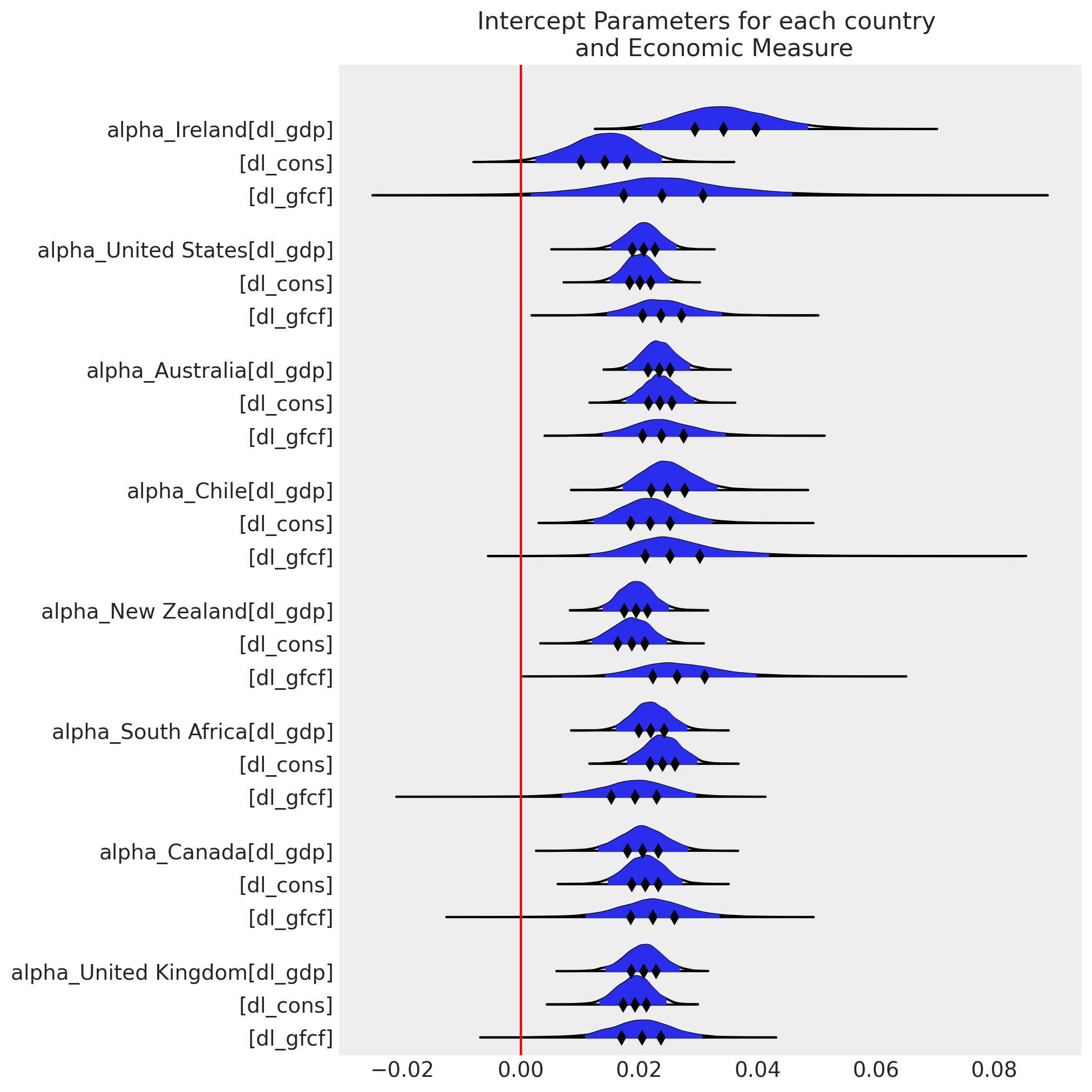
../_images/708fa57bc05b287a439ac2eca09319f05ef5d305b9ee154e8d123d4218038f75.png

ax = az.plot_forest(
    idata_full_test,
    var_names=[
        "lag_coefs_Ireland",
        "lag_coefs_United States",
        "lag_coefs_Australia",
        "lag_coefs_Chile",
        "lag_coefs_New Zealand",
        "lag_coefs_South Africa",
        "lag_coefs_Canada",
        "lag_coefs_United Kingdom",
    ],
    kind="ridgeplot",
    ridgeplot_truncate=False,
    figsize=(10, 10),
    coords={"equations": "dl_cons", "lags": 1, "cross_vars": "dl_gdp"},
)
ax[0].axvline(0, color="red")
ax[0].set_title("Lag Coefficient for the first lag of GDP on Consumption \n by Country");

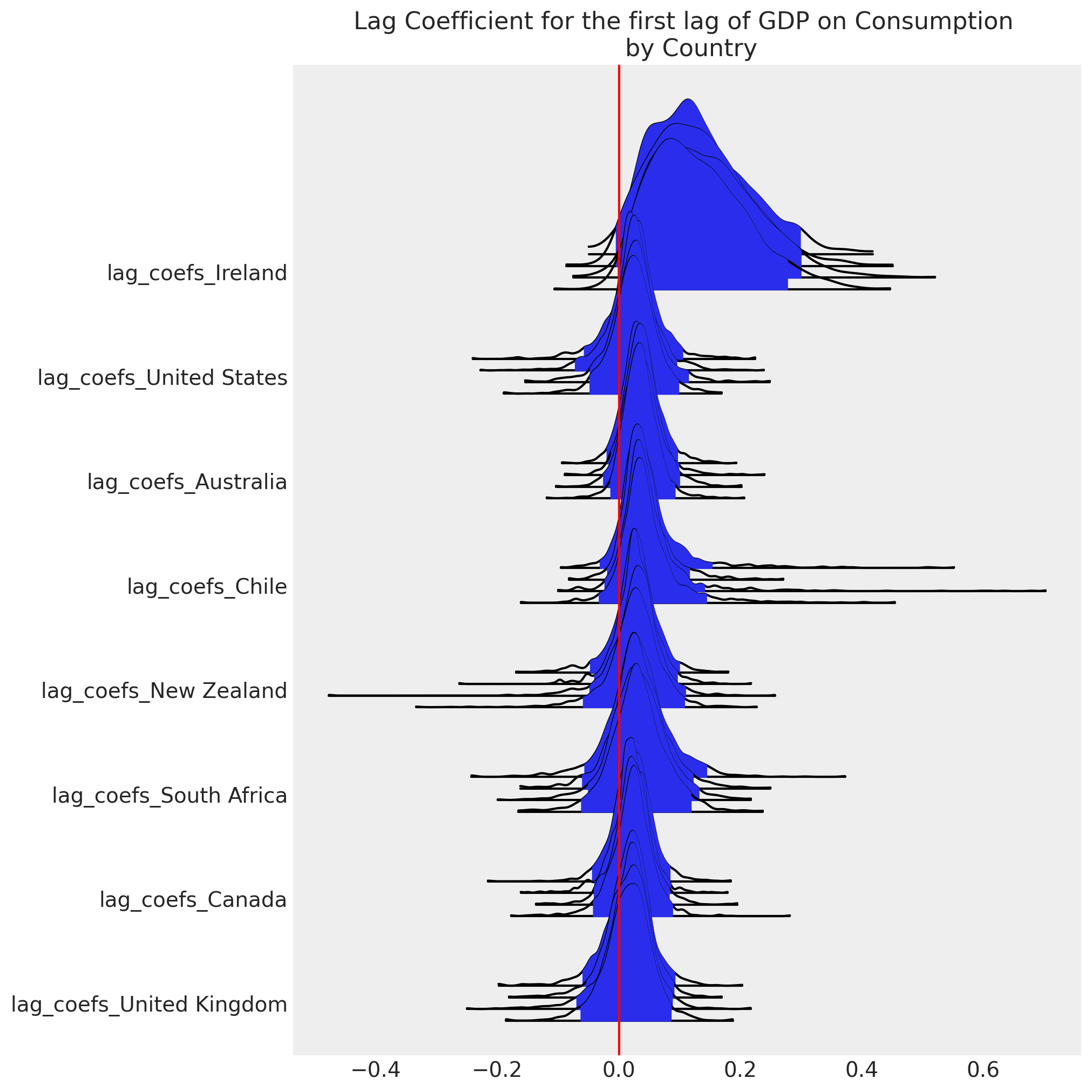
../_images/f4266cc9962e37d1182e4cf1b48f5c995454b0223a7dd632eaa918b646cabf0a.png

接下来我们将检查三个变量之间的相关性，看看通过包含分层结构我们学到了什么。

corr = pd.DataFrame(
    az.summary(idata_full_test, var_names=["omega_global_corr"])["mean"].values.reshape(3, 3),
    columns=["GDP", "CONS", "GFCF"],
)
corr.index = ["GDP", "CONS", "GFCF"]
corr

/Users/nathanielforde/mambaforge/envs/myjlabenv/lib/python3.11/site-packages/arviz/stats/diagnostics.py:584: RuntimeWarning: invalid value encountered in scalar divide
  (between_chain_variance / within_chain_variance + num_samples - 1) / (num_samples)

	GDP	CONS	GFCF
GDP	1.000	0.980	0.916
CONS	0.980	1.000	0.879
GFCF	0.916	0.879	1.000

ax = az.plot_posterior(
    idata_full_test,
    var_names="omega_global_corr",
    hdi_prob="hide",
    point_estimate="mean",
    grid=(3, 3),
    kind="hist",
    ec="black",
    figsize=(10, 7),
)
titles = [
    "GDP/GDP",
    "GDP/CONS",
    "GDP/GFCF",
    "CONS/GDP",
    "CONS/CONS",
    "CONS/GFCF",
    "GFCF/GDP",
    "GFCF/CONS",
    "GFCF/GFCF",
]
for ax, t in zip(ax.ravel(), titles):
    ax.set_xlim(0.6, 1)
    ax.set_title(t, fontsize=10)
plt.suptitle("The Posterior Correlation Estimates", fontsize=20);

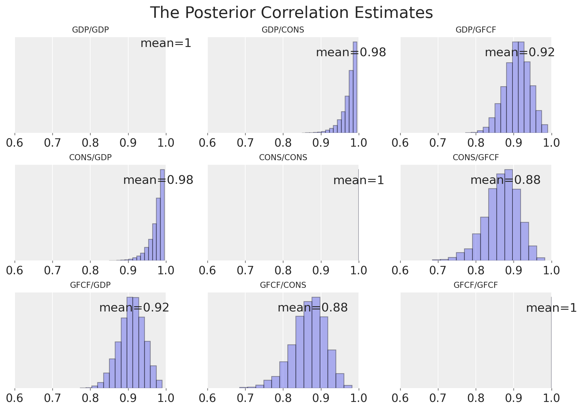
../_images/a9a547cae3a8bbee1dd7a1b0d7e2ee8c0291636e99c8a8cf17d4a6c6935367bf.png

我们可以看到，这三个经济变量之间相关性的估计值与我们单独研究爱尔兰的简单情况有显著差异。特别是，我们可以看到 GDF 和 CONS 之间的相关性现在更高了。这表明我们已经了解了这些变量之间关系的一些信息，而这些信息在单独研究爱尔兰案例时并不明显。

接下来我们将绘制每个国家的模型拟合图，以确保预测分布能够恢复观测数据。对于模型充分性的问题，重要的是我们既能恢复爱尔兰的异常值情况，也能恢复澳大利亚和美国等更常规国家的情况。

az.plot_ppc(idata_full_test);

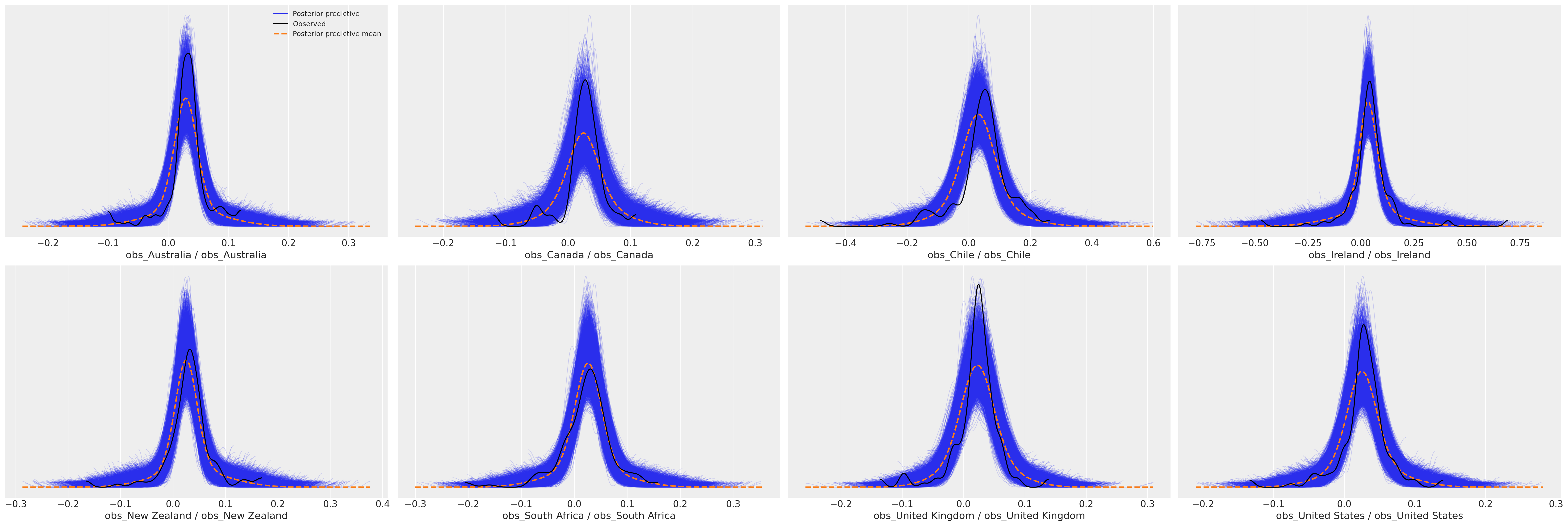
../_images/7a35a2c85b92acdda41eba93f1ac78df2f1eb882a02229d33a76dbd30ff4153c.png

为了查看这些模型拟合随时间的演变

countries = gdp_hierarchical["country"].unique()


fig, axs = plt.subplots(8, 3, figsize=(20, 40))
for ax, country in zip(axs, countries):
    temp = pd.DataFrame(
        idata_full_test["observed_data"][f"obs_{country}"].data,
        columns=["dl_gdp", "dl_cons", "dl_gfcf"],
    )
    ppc = az.extract(idata_full_test, group="posterior_predictive", num_samples=100)[
        f"obs_{country}"
    ]
    if country == "Ireland":
        color = "viridis"
    else:
        color = "inferno"
    for i in range(3):
        shade_background(ppc, ax, i, color)
    ax[0].plot(np.arange(ppc.shape[0]), ppc[:, 0, :].mean(axis=1), color="cyan", label="Mean")
    ax[0].plot(temp["dl_gdp"], "o", mfc="black", mec="white", mew=1, markersize=7, label="Observed")
    ax[0].set_title(f"Posterior Predictive GDP: {country}")
    ax[0].legend(loc="lower left")
    ax[1].plot(
        temp["dl_cons"], "o", mfc="black", mec="white", mew=1, markersize=7, label="Observed"
    )
    ax[1].plot(np.arange(ppc.shape[0]), ppc[:, 1, :].mean(axis=1), color="cyan", label="Mean")
    ax[1].set_title(f"Posterior Predictive Consumption: {country}")
    ax[1].legend(loc="lower left")
    ax[2].plot(
        temp["dl_gfcf"], "o", mfc="black", mec="white", mew=1, markersize=7, label="Observed"
    )
    ax[2].plot(np.arange(ppc.shape[0]), ppc[:, 2, :].mean(axis=1), color="cyan", label="Mean")
    ax[2].set_title(f"Posterior Predictive Investment: {country}")
    ax[2].legend(loc="lower left")
plt.suptitle("Posterior Predictive Checks on Hierarchical VAR", fontsize=20);

../_images/24c70f66bf4247625c0651c404b9457dd1390ba05e1dd1d1e07485f64e71acd5.png

在这里我们可以看到，该模型似乎已经恢复了观测数据的合理后验预测，并且与其他国家相比，爱尔兰 GDP 数据的波动性非常明显。这是否是关于数据质量还是指标被破坏的警示故事，我们留给经济学家来弄清楚。

结论#

VAR 模型构建是经济学中一个丰富而有趣的研究领域，在这些模型的解释和理解方面存在一系列挑战和陷阱。我们希望这个例子能够鼓励您继续探索贝叶斯框架中此类 VAR 模型构建的潜力。无论您是对宏观经济理论之间的关系感兴趣，还是对不良应用程序性能对客户反馈的影响等更简单的问题感兴趣，VAR 模型都为您提供了一个强大的工具，用于随着时间的推移探究这些关系。正如我们所看到的，分层 VAR 进一步实现了对同类群组中异常值的精确量化，并且不会因为国际资本主义产生的奇怪会计实务而丢弃信息。

在本系列的下一篇文章中，我们将花一些时间深入研究拟合 VAR 模型后得到的时间序列之间隐含的关系。

参考文献#

[1]

Ricardo Vieira。PyMC 中的贝叶斯向量自回归。URL: https://www.pymc-labs.io/blog-posts/bayesian-vector-autoregression/ (访问于 2022-12-09)。

作者#

改编自 PYMC labs 博客文章和 Jim Savage 的讨论这里，由 Nathaniel Forde 于 2022 年 11 月完成 (pymc-examples#456)
由 Nathaniel Forde 于 2023 年 2 月重新执行 (pymc_examples#523)

水印#

%load_ext watermark
%watermark -n -u -v -iv -w -p pytensor,aeppl,xarray

Last updated: Tue Feb 21 2023

Python implementation: CPython
Python version       : 3.11.0
IPython version      : 8.9.0

pytensor: 2.8.11
aeppl   : not installed
xarray  : 2023.1.0

pymc       : 5.0.1
statsmodels: 0.13.5
pandas     : 1.5.3
numpy      : 1.24.1
matplotlib : 3.6.3
arviz      : 0.14.0

Watermark: 2.3.1

许可声明#

本示例库中的所有笔记本均根据 MIT 许可证提供，该许可证允许修改和再分发以用于任何用途，前提是版权和许可声明得到保留。

引用 PyMC 示例#

要引用此笔记本，请使用 Zenodo 为 pymc-examples 存储库提供的 DOI。

重要

许多笔记本改编自其他来源：博客、书籍…… 在这种情况下，您也应该引用原始来源。

另请记住引用代码中使用的相关库。

这是一个 bibtex 中的引用模板

@incollection{citekey,
  author    = "<notebook authors, see above>",
  title     = "<notebook title>",
  editor    = "PyMC Team",
  booktitle = "PyMC examples",
  doi       = "10.5281/zenodo.5654871"
}

渲染后可能看起来像

分类

标签