随机波动率模型

import os

import arviz as az
import matplotlib.pyplot as plt
import numpy as np
import pandas as pd
import pymc as pm

rng = np.random.RandomState(1234)
az.style.use("arviz-darkgrid")

资产价格具有随时间变化的波动性（日收益率的方差）。在某些时期，收益率波动很大，而在另一些时期则非常稳定。随机波动率模型使用潜在的波动率变量对此进行建模，该变量被建模为随机过程。以下模型类似于 No-U-Turn Sampler 论文中描述的模型，[Hoffman 和 Gelman, 2014]。

\[ \sigma \sim Exponential(50) \]

\[ \nu \sim Exponential(.1) \]

\[ s_i \sim Normal(s_{i-1}, \sigma^{-2}) \]

\[ \log(r_i) \sim t(\nu, 0, \exp(-2 s_i)) \]

这里，\(r\) 是每日收益率序列，\(s\) 是潜在的对数波动率过程。

构建模型

首先，我们加载标准普尔 500 指数的每日收益率，并计算每日对数收益率。此数据来自 2008 年 5 月至 2019 年 11 月。

try:
    returns = pd.read_csv(os.path.join("..", "data", "SP500.csv"), index_col="Date")
except FileNotFoundError:
    returns = pd.read_csv(pm.get_data("SP500.csv"), index_col="Date")

returns["change"] = np.log(returns["Close"]).diff()
returns = returns.dropna()

returns.head()

	收盘价	变化
日期
2008-05-05	1407.489990	-0.004544
2008-05-06	1418.260010	0.007623
2008-05-07	1392.569946	-0.018280
2008-05-08	1397.680054	0.003663
2008-05-09	1388.280029	-0.006748

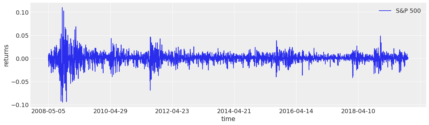
如您所见，波动性似乎随时间变化很大，但聚集在某些时间段附近。例如，2008 年的金融危机很容易辨认出来。

fig, ax = plt.subplots(figsize=(14, 4))
returns.plot(y="change", label="S&P 500", ax=ax)
ax.set(xlabel="time", ylabel="returns")
ax.legend();

在 PyMC 中指定模型反映了其统计规范。

def make_stochastic_volatility_model(data):
    with pm.Model(coords={"time": data.index.values}) as model:
        step_size = pm.Exponential("step_size", 10)
        volatility = pm.GaussianRandomWalk(
            "volatility", sigma=step_size, dims="time", init_dist=pm.Normal.dist(0, 100)
        )
        nu = pm.Exponential("nu", 0.1)
        returns = pm.StudentT(
            "returns", nu=nu, lam=np.exp(-2 * volatility), observed=data["change"], dims="time"
        )
    return model


stochastic_vol_model = make_stochastic_volatility_model(returns)

检查模型

确保我们的模型符合预期的两个好方法是：

1. 查看模型结构。这让我们知道我们指定了想要的先验和想要的连接。它也有助于提醒我们随机变量的大小。

2. 查看先验预测样本。这有助于我们解释先验对数据的暗示。

pm.model_to_graphviz(stochastic_vol_model)

with stochastic_vol_model:
    idata = pm.sample_prior_predictive(500, random_seed=rng)

prior_predictive = az.extract(idata, group="prior_predictive")

Sampling: [nu, returns, step_size, volatility]

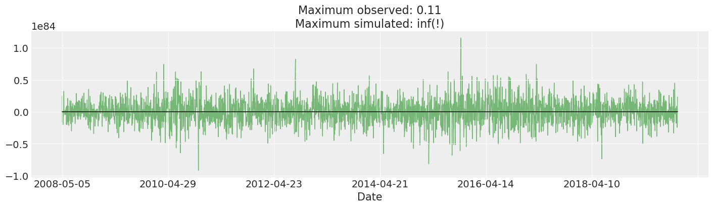
我们绘制并检查先验预测。这比我们观察到的实际收益率大许多数量级。实际上，我特意挑选了一些抽样，以防止图看起来很傻。这可能表明需要更改我们的先验：我们的模型认为合理的收益率将以巨大的幅度违反各种约束：世界生产的所有商品和服务的总价值约为 \(\$10^9\)，因此我们可能有理由不期望任何高于该数量级的收益率。

尽管如此，我们仍然得到了拟合此模型的相当合理的结果，并且它是标准的，因此我们保持原样。

fig, ax = plt.subplots(figsize=(14, 4))
returns["change"].plot(ax=ax, lw=1, color="black")
ax.plot(
    prior_predictive["returns"][:, 0::10],
    "g",
    alpha=0.5,
    lw=1,
    zorder=-10,
)

max_observed, max_simulated = np.max(np.abs(returns["change"])), np.max(
    np.abs(prior_predictive["returns"].values)
)
ax.set_title(f"Maximum observed: {max_observed:.2g}\nMaximum simulated: {max_simulated:.2g}(!)");

拟合模型

在我们对模型感到满意后，我们可以从后验分布中抽样。即使使用 NUTS，这也是一个有点棘手的模型，因此我们抽样和调整的时间比默认时间稍长。

with stochastic_vol_model:
    idata.extend(pm.sample(random_seed=rng))

posterior = az.extract(idata)
posterior["exp_volatility"] = np.exp(posterior["volatility"])

100.00% [8000/8000 01:52<00:00 采样 4 条链, 0 个发散]

Sampling 4 chains for 1_000 tune and 1_000 draw iterations (4_000 + 4_000 draws total) took 113 seconds.

with stochastic_vol_model:
    idata.extend(pm.sample_posterior_predictive(idata, random_seed=rng))

posterior_predictive = az.extract(idata, group="posterior_predictive")

100.00% [4000/4000 00:00<00:00]

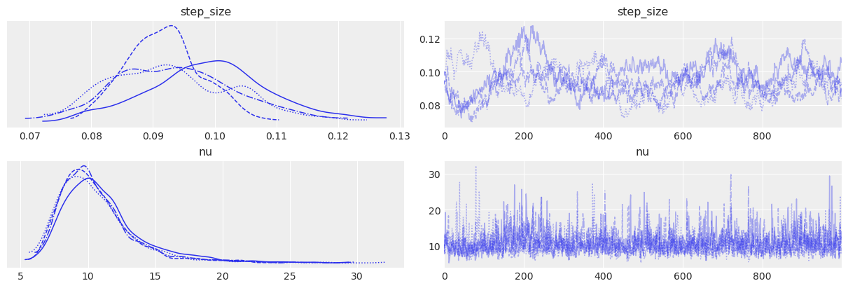
请注意，step_size 参数看起来不太完美：不同的链看起来有些不同。这再次表明我们模型存在一些弱点：允许步长随时间变化可能是有意义的，尤其是在这 11 年的时间跨度内。

az.plot_trace(idata, var_names=["step_size", "nu"]);

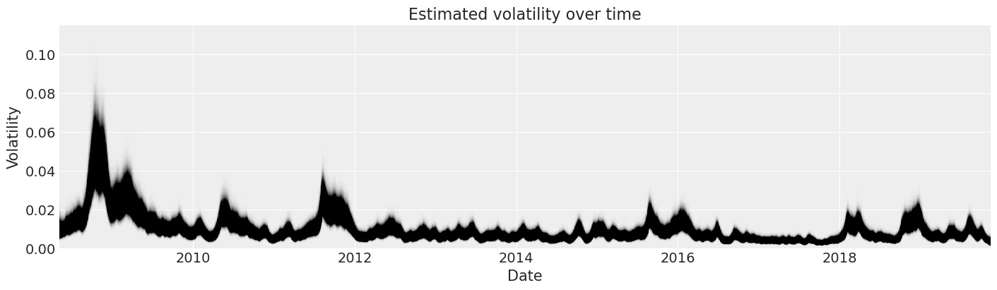
现在我们可以查看我们对标准普尔 500 指数收益率随时间变化的波动性的后验估计。

fig, ax = plt.subplots(figsize=(14, 4))

y_vals = posterior["exp_volatility"]
x_vals = y_vals.time.astype(np.datetime64)

plt.plot(x_vals, y_vals, "k", alpha=0.002)
ax.set_xlim(x_vals.min(), x_vals.max())
ax.set_ylim(bottom=0)
ax.set(title="Estimated volatility over time", xlabel="Date", ylabel="Volatility");

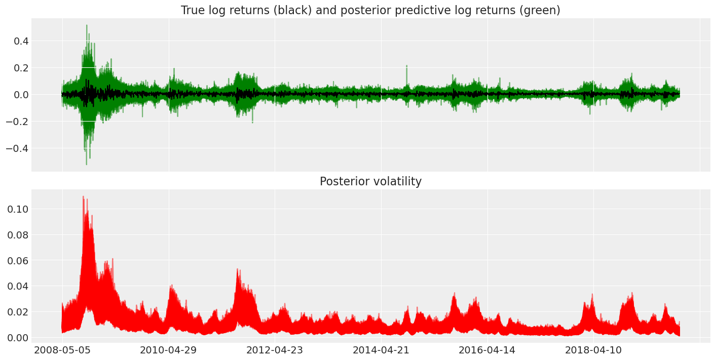
最后，我们可以使用后验预测分布来查看学习到的波动性如何影响收益率。

fig, axes = plt.subplots(nrows=2, figsize=(14, 7), sharex=True)
returns["change"].plot(ax=axes[0], color="black")

axes[1].plot(posterior["exp_volatility"], "r", alpha=0.5)
axes[0].plot(
    posterior_predictive["returns"],
    "g",
    alpha=0.5,
    zorder=-10,
)
axes[0].set_title("True log returns (black) and posterior predictive log returns (green)")
axes[1].set_title("Posterior volatility");

%load_ext watermark
%watermark -n -u -v -iv -w -p pytensor,aeppl,xarray

Last updated: Sun Feb 05 2023

Python implementation: CPython
Python version       : 3.10.9
IPython version      : 8.9.0

pytensor: 2.8.11
aeppl   : not installed
xarray  : 2023.1.0

arviz     : 0.14.0
pymc      : 5.0.1
matplotlib: 3.6.3
numpy     : 1.24.1
pandas    : 1.5.3

Watermark: 2.3.1

参考文献

[1]

Matthew Hoffman 和 Andrew Gelman. The no-u-turn sampler: adaptively setting path lengths in hamiltonian monte carlo. Journal of Machine Learning Research, 15:1593–1623, 2014. URL: https://dl.acm.org/doi/10.5555/2627435.2638586.

作者

• 作者：John Salvatier

• 更新者：Kyle Meyer

• 更新者：Thomas Wiecki

• 更新者：Chris Fonnesbeck

• 更新者：Aaron Maxwell，于 2018 年 5 月 18 日 (pymc#2978)

• 更新者：Colin Carroll，于 2019 年 11 月 16 日 (pymc#3682)

• 更新者：Abhipsha Das，于 2021 年 7 月 24 日 (pymc-examples#155)

• 更新者：Michael Osthege，于 2022 年 6 月 1 日 (pymc-examples#343)

• 更新者：Christopher Krapu，于 2022 年 6 月 17 日 (pymc-examples#378)

• 更新者：Beryl Kanali 和 Sangam Swadik，于 2023 年 1 月 22 日，与 PyMC v5 兼容 (pymc-examples#517)

• 更新者：Benjamin T. Vincent，使用 az.extract (pymc-examples#522)

许可声明

本示例库中的所有笔记本均根据 MIT 许可证 提供，该许可证允许修改和再分发以用于任何用途，前提是保留版权和许可声明。

引用 PyMC 示例

要引用此笔记本，请使用 Zenodo 为 pymc-examples 存储库提供的 DOI。

重要提示

许多笔记本改编自其他来源：博客、书籍……在这种情况下，您也应该引用原始来源。

另请记住引用您的代码使用的相关库。

这是一个 bibtex 格式的引用模板

@incollection{citekey,
  author    = "<notebook authors, see above>",
  title     = "<notebook title>",
  editor    = "PyMC Team",
  booktitle = "PyMC examples",
  doi       = "10.5281/zenodo.5654871"
}

渲染后可能如下所示