


广义极值分布#
简介#
广义极值 (GEV) 分布是一个元分布,包含威布尔分布、耿贝尔分布和弗雷歇分布族。它用于对平稳过程的极值(最大值或最小值)分布进行建模,例如年度最大风速、桥梁上的年度最大卡车重量等等,而无需先验决定尾部行为。
根据 Coles [2001] 中使用的参数化,最大值的 GEV 分布由下式给出
当
\(\xi < 0\) 我们得到具有有界上尾的威布尔分布;
\(\xi = 0\),在极限情况下,我们得到耿贝尔分布,在两个尾部都是无界的;
\(\xi > 0\),我们得到弗雷歇分布,它在下尾是有界的。
请注意,形状参数 \(\xi\) 的这种参数化与 SciPy 中使用的符号相反(在 SciPy 中它表示为 c)。此外,通过研究数据负数的最大值分布,可以很容易地检查最小值的分布。
我们将使用 Coles [2001] 中使用的 Port Pirie 年度最大海平面数据的示例,并与其中提供的频率学结果进行比较。
import arviz as az
import matplotlib.pyplot as plt
import numpy as np
import pymc as pm
import pymc_extras.distributions as pmx
import pytensor.tensor as pt

from arviz.plots import plot_utils as azpu
数据#
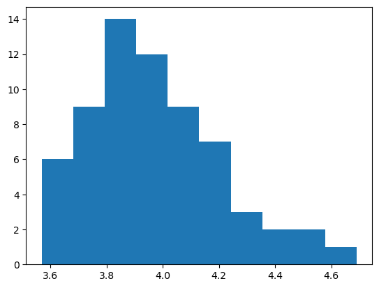
Port Pirie 数据由 Coles [2001] 提供,并在此处重复
# fmt: off
data = np.array([4.03, 3.83, 3.65, 3.88, 4.01, 4.08, 4.18, 3.80,
                 4.36, 3.96, 3.98, 4.69, 3.85, 3.96, 3.85, 3.93,
                 3.75, 3.63, 3.57, 4.25, 3.97, 4.05, 4.24, 4.22,
                 3.73, 4.37, 4.06, 3.71, 3.96, 4.06, 4.55, 3.79,
                 3.89, 4.11, 3.85, 3.86, 3.86, 4.21, 4.01, 4.11,
                 4.24, 3.96, 4.21, 3.74, 3.85, 3.88, 3.66, 4.11,
                 3.71, 4.18, 3.90, 3.78, 3.91, 3.72, 4.00, 3.66,
                 3.62, 4.33, 4.55, 3.75, 4.08, 3.90, 3.88, 3.94,
                 4.33])
# fmt: on
plt.hist(data)
plt.show()
建模与预测#
在建模中,我们希望做两件事
基于一些相当非信息性的先验,对 GEV 参数进行参数推断,以及;
预测 10 年重现期水平。
在贝叶斯设置中,可以轻松完成考虑参数不确定性的极值预测。有趣的是,将这种简易性与 Caprani 和 OBrien [2010] 在频率学设置中执行此操作时遇到的困难进行比较。在任何情况下,概率超出 \(p\) 的预测值由下式给出
这是一个参数值的确定性函数,因此使用模型上下文中的 pm.Deterministic 完成。
然后考虑 10 年重现期,其中 \(p = 1/10\)
p = 1 / 10
现在使用从上面直方图的快速回顾中估计的先验来设置模型
\(\mu\):除了标准差限制负面结果的
Normal分布之外,没有真正的理由考虑其他任何分布;\(\sigma\):这必须是正数,并且值很小,因此使用具有单位标准差的
HalfNormal;\(\xi\):我们对尾部行为持不可知态度,因此将其中心设为零,但限制在 \(\pm 0.6\) 的物理合理范围内,并使其在零附近保持某种程度的紧密。
# Optionally centre the data, depending on fitting and divergences
# cdata = (data - data.mean())/data.std()

with pm.Model() as model:
    # Priors
    μ = pm.Normal("μ", mu=3.8, sigma=0.2)
    σ = pm.HalfNormal("σ", sigma=0.3)
    ξ = pm.TruncatedNormal("ξ", mu=0, sigma=0.2, lower=-0.6, upper=0.6)

    # Estimation
    gev = pmx.GenExtreme("gev", mu=μ, sigma=σ, xi=ξ, observed=data)
    # Return level
    z_p = pm.Deterministic("z_p", μ - σ / ξ * (1 - (-np.log(1 - p)) ** (-ξ)))
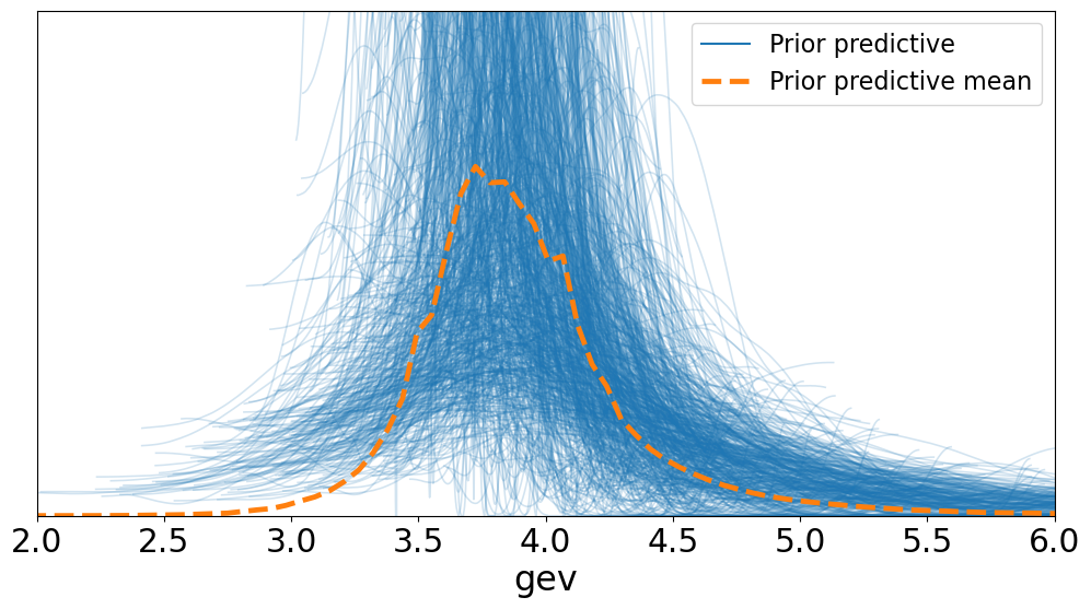
先验预测检查#
让我们感受一下我们选择的先验如何很好地覆盖数据范围
idata = pm.sample_prior_predictive(samples=1000, model=model)
az.plot_ppc(idata, group="prior", figsize=(12, 6))
ax = plt.gca()
ax.set_xlim([2, 6])
ax.set_ylim([0, 2]);
Sampling: [gev, μ, ξ, σ]
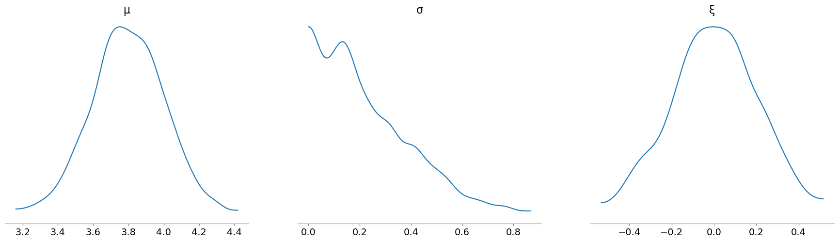
我们可以使用 plot_posterior 函数查看参数的抽样值,但传入 idata 对象并指定 group 为 "prior"
az.plot_posterior(
    idata, group="prior", var_names=["μ", "σ", "ξ"], hdi_prob="hide", point_estimate=None
);
推断#
按下神奇的推断按钮\(^{\mathrm{TM}}\)
with model:
    trace = pm.sample(
        5000,
        cores=4,
        chains=4,
        tune=2000,
        initvals={"μ": -0.5, "σ": 1.0, "ξ": -0.1},
        target_accept=0.98,
    )
# add trace to existing idata object
idata.extend(trace)
Initializing NUTS using jitter+adapt_diag...
Multiprocess sampling (4 chains in 4 jobs)
NUTS: [μ, σ, ξ]
Sampling 4 chains for 2_000 tune and 5_000 draw iterations (8_000 + 20_000 draws total) took 4 seconds.
There were 19 divergences after tuning. Increase `target_accept` or reparameterize.
az.plot_trace(idata, var_names=["μ", "σ", "ξ"], figsize=(12, 12));
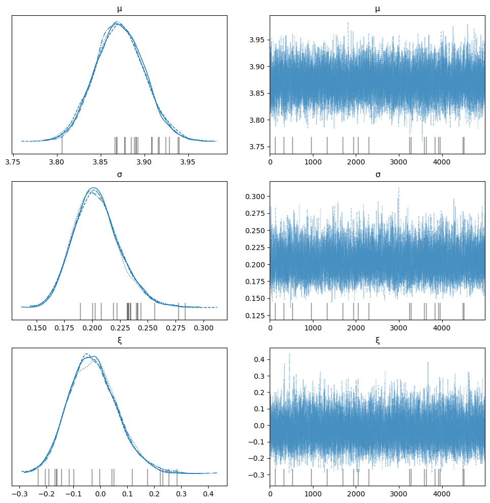
发散#
迹线表现出发散(通常)。当参数的支持边界接近时,HMC/NUTS 采样器可能会出现问题。并且由于 GEV 的边界随 \(\xi\) 的符号而变化,因此很难提供解决此问题的转换。 Bali [2003] 提出了一个可能的转换 - Box-Cox 转换,但 Caprani 和 OBrien [2010] 发现即使对于最大似然估计,它在数值上也是不稳定的。在任何情况下,缓解发散问题的建议是
增加目标接受率;
使用更多信息性的先验,特别是将形状参数限制在物理合理的值范围内,通常为 \(\xi \in [-0.5,0.5]\);
确定尾部的吸引域(即威布尔分布、耿贝尔分布或弗雷歇分布),并直接使用该分布。
推断结果#
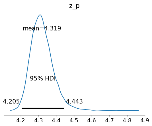
参数估计的 95% 可信区间范围是
az.hdi(idata, hdi_prob=0.95)
<xarray.Dataset> Size: 112B
Dimensions:  (hdi: 2)
Coordinates:
  * hdi      (hdi) <U6 48B 'lower' 'higher'
Data variables:
    z_p      (hdi) float64 16B 4.205 4.443
    μ        (hdi) float64 16B 3.818 3.927
    ξ        (hdi) float64 16B -0.1967 0.1532
σ (hdi) float64 16B 0.1649 0.246并检查预测分布,考虑参数变异性(并且无需假设正态性)
az.plot_posterior(idata, hdi_prob=0.95, var_names=["z_p"], round_to=4);
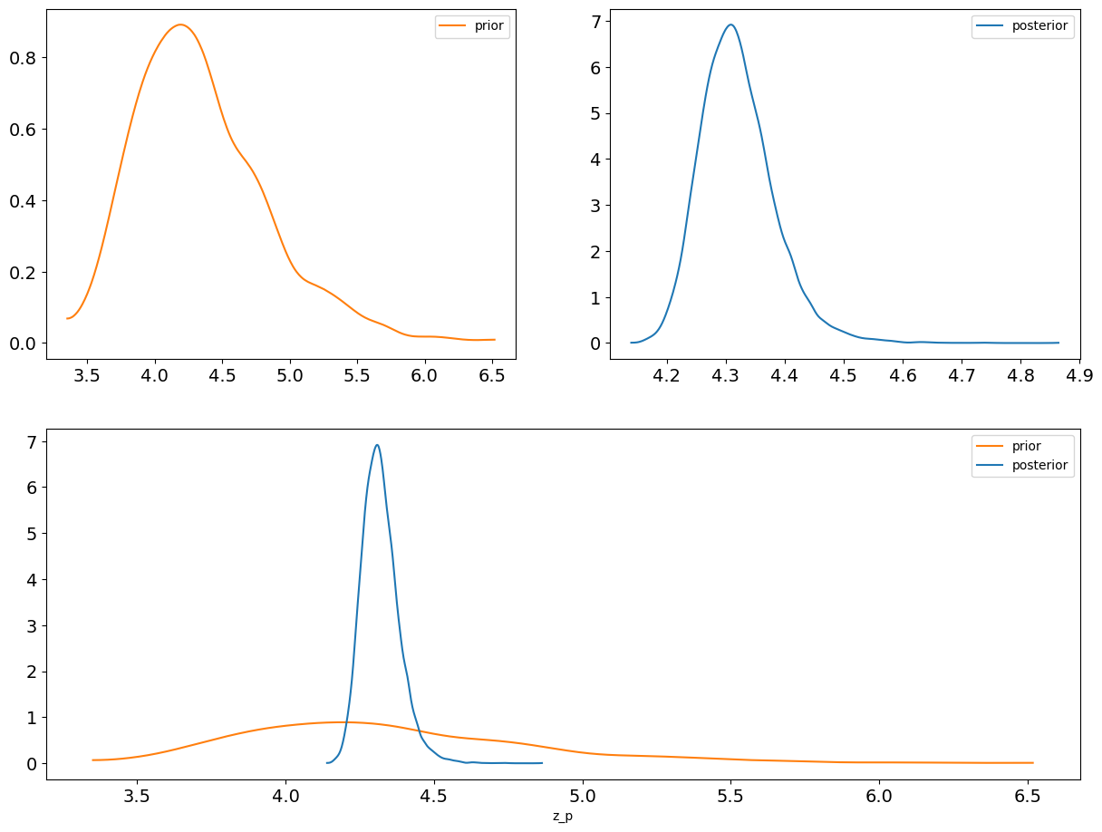
让我们比较 \(z_p\) 的先验和后验预测,看看数据如何影响结果
az.plot_dist_comparison(idata, var_names=["z_p"]);
比较#
为了与 Coles [2001] 中给出的结果进行比较,我们使用后验分布的众数(最大后验或 MAP 估计)来近似最大似然估计 (MLE)。当先验在后验估计附近相当平坦时,这些值会很接近。
Coles [2001] 中给出的 MLE 结果是
估计的方差-协方差矩阵为
请注意,从我们的推断中提取 MLE 估计涉及访问一些 Arviz 后端函数,以将 xarray 转换为可检查的内容
_, vals = az.sel_utils.xarray_to_ndarray(idata["posterior"], var_names=["μ", "σ", "ξ"])
mle = [azpu.calculate_point_estimate("mode", val) for val in vals]
mle
[3.870336499417071, 0.19875954328704448, -0.05287169063589742]
idata["posterior"].drop_vars("z_p").to_dataframe().cov().round(6)
| μ | ξ | σ | |
|---|---|---|---|
| μ | 0.000778 | -0.000766 | 0.000179 |
| ξ | -0.000766 | 0.008066 | -0.000553 |
| σ | 0.000179 | -0.000553 | 0.000436 |
结果非常吻合,但在贝叶斯设置中执行此操作的好处是,我们几乎免费获得了参数和重现期的完整后验联合分布。将其与松散的正态性假设和计算工作量进行比较,以获得甚至方差-协方差矩阵,如 Coles [2001] 中所做的那样。
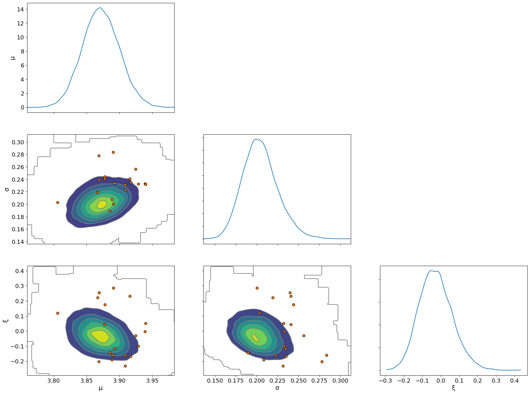
最后,我们检查成对图,并查看使用发散的推断中的任何困难
az.plot_pair(idata, var_names=["μ", "σ", "ξ"], kind="kde", marginals=True, divergences=True);
参考文献#
Stuart Coles. An introduction to statistical modeling of extreme values. Springer Series in Statistics. Springer, London, England, 2001 edition, August 2001. ISBN 978-1-85233-459-8. URL: https://doi.org/10.1007/978-1-4471-3675-0.
Colin C. Caprani 和 Eugene J. OBrien. The use of predictive likelihood to estimate the distribution of extreme bridge traffic load effect. Structural Safety, 32(2):138–144, 2010. URL: https://www.sciencedirect.com/science/article/pii/S016747300900071X, doi:https://doi.org/10.1016/j.strusafe.2009.09.001.
Turan G. Bali. The generalized extreme value distribution. Economics Letters, 79(3):423–427, 2003. URL: https://www.sciencedirect.com/science/article/pii/S0165176503000351, doi:https://doi.org/10.1016/S0165-1765(03)00035-1.
Colin C. Caprani 和 Eugene J. OBrien. Estimating extreme highway bridge traffic load effects. In Hitoshi Furuta, Dan M Frangopol, and Masanobu Shinozuka, editors, Proceedings of the 10th International Conference on Structural Safety and Reliability (ICOSSAR2009), 1 – 8. CRC Press, 2010. URL: https://citeseerx.ist.psu.edu/viewdoc/download?doi=10.1.1.722.6789\&rep=rep1\&type=pdf.
水印#
%load_ext watermark
%watermark -n -u -v -iv -w -p pytensor,arviz
Last updated: Sat Dec 14 2024

Python implementation: CPython
Python version       : 3.12.5
IPython version      : 8.27.0

pytensor: 2.26.4
arviz   : 0.19.0

matplotlib : 3.9.2
numpy      : 1.26.4
pymc       : 5.19.1
arviz      : 0.19.0
pytensor   : 2.26.4
pymc_extras: 0.2.0

Watermark: 2.5.0