


离散选择和随机效用模型#
注意
此笔记本使用非 PyMC 依赖项的库,因此需要专门安装才能运行此笔记本。打开下面的下拉菜单以获得更多指导。
额外的依赖项安装说明
为了运行此笔记本(在本地或 Binder 上),您不仅需要安装可用的 PyMC 以及所有可选依赖项,还需要安装一些额外的依赖项。有关安装 PyMC 本身的建议,请参阅安装
您可以使用您首选的包管理器安装这些依赖项,我们提供以下 pip 和 conda 命令作为示例。
$ pip install jax, jaxlib, numpyro
请注意,如果您想(或需要)从笔记本内部而不是命令行安装软件包,您可以通过运行 pip 命令的变体来安装软件包
import sys
!{sys.executable} -m pip install jax, jaxlib, numpyro
您不应运行 !pip install,因为它可能会将软件包安装在不同的环境中,即使已安装,也无法从 Jupyter 笔记本中使用。
另一种选择是使用 conda 代替
$ conda install jax, jaxlib, numpyro
当使用 conda 安装科学 python 包时,我们建议使用 conda forge
import arviz as az
import numpy as np  # For vectorized math operations
import pandas as pd  # For file input/output
import pymc as pm
import pytensor.tensor as pt

from matplotlib import pyplot as plt
from matplotlib.lines import Line2D
%config InlineBackend.figure_format = 'retina'  # high resolution figures
az.style.use("arviz-darkgrid")
rng = np.random.default_rng(42)
离散选择建模:理念#
离散选择建模与有序分类结果的回归模型中讨论的潜在效用尺度的概念相关,但它将该概念推广到决策制定。它假设人类决策制定可以建模为一组互斥备选方案的潜在/主观效用测量的函数。该理论指出,任何决策者都会选择最大化其主观效用的选项,并且效用可以建模为世界可观察特征的潜在线性函数。
丹尼尔·麦克法登在 1970 年代最著名地应用了这一理念,以预测拟议引入 BART 轻轨系统后,加利福尼亚州交通方式选择(即汽车、铁路、步行等)的市场份额。值得在此停顿一下。该理论是关于微观层面的人类决策制定,在实际应用中,已扩展到做出大致准确的宏观层面预测。有关更多详细信息,我们推荐 Train [2009]
我们也不需要过于轻信。这仅仅是一个统计模型,这里的成功完全取决于建模者的技能和可用的测量,以及合理的理论。但值得注意的是这些模型背后的雄心壮志。模型的结构鼓励您阐明您对决策者及其所处环境的理论。
数据#
在此示例中,我们将使用 (i) 来自 R mlogit 包的供暖系统数据集和 (ii) 跨饼干品牌的重复选择数据集来检验离散选择建模技术。我们将采用贝叶斯方法来估计模型,而不是其 vignette 中报告的 MLE 方法。第一个数据集显示了加利福尼亚州家庭对供暖系统报价的选择。观测对象是加利福尼亚州新建的且装有中央空调的独户住宅。考虑了五种可能的系统类型
燃气中央供暖 (gc),
燃气室式供暖 (gr),
电力中央供暖 (ec),
电力室式供暖 (er),
热泵 (hp)。
该数据集报告了每个家庭面临的五种备选方案的安装成本 ic.alt 和运营成本 oc.alt,以及关于家庭的一些广泛的人口统计信息,以及至关重要的选择 depvar。这是一个选择场景中五种备选方案在数据中的样子
try:
    wide_heating_df = pd.read_csv("../data/heating_data_r.csv")
except:
    wide_heating_df = pd.read_csv(pm.get_data("heating_data_r.csv"))

wide_heating_df[wide_heating_df["idcase"] == 1]
| idcase | depvar | ic.gc | ic.gr | ic.ec | ic.er | ic.hp | oc.gc | oc.gr | oc.ec | oc.er | oc.hp | income | agehed | rooms | region | |
|---|---|---|---|---|---|---|---|---|---|---|---|---|---|---|---|---|
| 0 | 1 | gc | 866.0 | 962.64 | 859.9 | 995.76 | 1135.5 | 199.69 | 151.72 | 553.34 | 505.6 | 237.88 | 7 | 25 | 6 | ncostl |
这些模型的中心思想是将此场景视为对具有附加潜在效用的详尽选项的选择。归因于每个选项的效用被视为每个选项属性的线性组合。归因于每个备选方案的效用驱动着在每个选项中进行选择的概率。对于所有备选方案 \(Alt = \{ gc, gr, ec, er, hp \}\) 中的每个 \(j\),假设其服从耿贝尔分布,因为这具有特别好的数学性质。
这个假设被证明在数学上很方便,因为两个耿贝尔分布之间的差异可以建模为逻辑函数,这意味着我们可以使用 softmax 函数对多个备选方案之间的对比差异进行建模。推导的详细信息可以在 Train [2009] 中找到
然后,该模型假设决策者选择最大化其主观效用的选项。个人效用函数可以进行丰富的参数化。只有当备选方案的效用测量值以“外部商品”的固定效用为基准时,模型才能被识别。最后一个量通常固定为 0,以帮助识别备选方案特定参数,我们将在下面看到。
应用所有这些约束后,我们可以构建条件随机效用模型及其分层变体。与统计学中的几乎所有主题一样,模型规范的精确词汇是过载的。条件 logit 参数 \(\beta\) 可以固定在个人层面,但可以在个人和备选方案 gc, gr, ec, er 之间变化。通过这种方式,我们可以构成一个详细的理论,说明我们期望主观效用的驱动因素如何改变一组竞争商品之间的市场份额。
关于数据格式的题外话#
离散选择模型通常使用长数据格式进行估计,其中每个选择场景都用每备选方案 ID 一行和一个二进制标志表示,该标志表示每个场景中选择的选项。建议使用此数据格式在 stan 和 pylogit 中估计这些类型的模型。这样做的原因是,一旦以这种方式透视了 installation_costs 和 operating_costs 列,就更容易将它们包含在矩阵计算中。
try:
    long_heating_df = pd.read_csv("../data/long_heating_data.csv")
except:
    long_heating_df = pd.read_csv(pm.get_data("long_heating_data.csv"))

columns = [c for c in long_heating_df.columns if c != "Unnamed: 0"]
long_heating_df[long_heating_df["idcase"] == 1][columns]
| idcase | alt_id | choice | depvar | income | agehed | rooms | region | installation_costs | operating_costs | |
|---|---|---|---|---|---|---|---|---|---|---|
| 0 | 1 | 1 | 1 | gc | 7 | 25 | 6 | ncostl | 866.00 | 199.69 |
| 1 | 1 | 2 | 0 | gc | 7 | 25 | 6 | ncostl | 962.64 | 151.72 |
| 2 | 1 | 3 | 0 | gc | 7 | 25 | 6 | ncostl | 859.90 | 553.34 |
| 3 | 1 | 4 | 0 | gc | 7 | 25 | 6 | ncostl | 995.76 | 505.60 |
| 4 | 1 | 5 | 0 | gc | 7 | 25 | 6 | ncostl | 1135.50 | 237.88 |
基本模型#
我们将在此处展示如何在 PyMC 中结合效用规范。PyMC 是此类建模的良好界面,因为它可以非常简洁地表达模型,遵循此方程组的自然数学表达式。您可以在这个简单的模型中看到我们如何分别构建每个备选方案的效用度量方程,然后将它们堆叠在一起,为我们的 softmax 变换创建输入矩阵。
N = wide_heating_df.shape[0]
observed = pd.Categorical(wide_heating_df["depvar"]).codes
coords = {
    "alts_probs": ["ec", "er", "gc", "gr", "hp"],
    "obs": range(N),
}

with pm.Model(coords=coords) as model_1:
    beta_ic = pm.Normal("beta_ic", 0, 1)
    beta_oc = pm.Normal("beta_oc", 0, 1)

    ## Construct Utility matrix and Pivot
    u0 = beta_ic * wide_heating_df["ic.ec"] + beta_oc * wide_heating_df["oc.ec"]
    u1 = beta_ic * wide_heating_df["ic.er"] + beta_oc * wide_heating_df["oc.er"]
    u2 = beta_ic * wide_heating_df["ic.gc"] + beta_oc * wide_heating_df["oc.gc"]
    u3 = beta_ic * wide_heating_df["ic.gr"] + beta_oc * wide_heating_df["oc.gr"]
    u4 = beta_ic * wide_heating_df["ic.hp"] + beta_oc * wide_heating_df["oc.hp"]
    s = pm.math.stack([u0, u1, u2, u3, u4]).T

    ## Apply Softmax Transform
    p_ = pm.Deterministic("p", pm.math.softmax(s, axis=1), dims=("obs", "alts_probs"))

    ## Likelihood
    choice_obs = pm.Categorical("y_cat", p=p_, observed=observed, dims="obs")

    idata_m1 = pm.sample_prior_predictive()
    idata_m1.extend(
        pm.sample(nuts_sampler="numpyro", idata_kwargs={"log_likelihood": True}, random_seed=101)
    )
    idata_m1.extend(pm.sample_posterior_predictive(idata_m1))

pm.model_to_graphviz(model_1)
Sampling: [beta_ic, beta_oc, y_cat]
/Users/nathanielforde/mambaforge/envs/pymc_examples_new/lib/python3.9/site-packages/pymc/sampling/mcmc.py:243: UserWarning: Use of external NUTS sampler is still experimental
  warnings.warn("Use of external NUTS sampler is still experimental", UserWarning)
Compiling...
Compilation time =  0:00:01.195286
Sampling...
Sampling time =  0:00:02.097556
Transforming variables...
Transformation time =  0:00:00.396818
Computing Log Likelihood...
Sampling: [y_cat]
Log Likelihood time = 0:00:00.638968

请注意,您需要小心结果变量的编码。分类顺序应反映效用堆叠到 softmax 变换中,然后馈送到似然项的顺序。
idata_m1
-
<xarray.Dataset> Dimensions: (chain: 4, draw: 1000, obs: 900, alts_probs: 5) Coordinates: * chain (chain) int64 0 1 2 3 * draw (draw) int64 0 1 2 3 4 5 6 7 ... 992 993 994 995 996 997 998 999 * obs (obs) int64 0 1 2 3 4 5 6 7 ... 892 893 894 895 896 897 898 899 * alts_probs (alts_probs) <U2 'ec' 'er' 'gc' 'gr' 'hp' Data variables: beta_ic (chain, draw) float64 -0.006063 -0.006218 ... -0.005608 beta_oc (chain, draw) float64 -0.004401 -0.00453 ... -0.004273 -0.004929 p (chain, draw, obs, alts_probs) float64 0.09993 ... 0.02927 Attributes: created_at: 2025-03-22T20:10:25.635782 arviz_version: 0.17.0 -
<xarray.Dataset> Dimensions: (chain: 4, draw: 1000, obs: 900) Coordinates: * chain (chain) int64 0 1 2 3 * draw (draw) int64 0 1 2 3 4 5 6 7 8 ... 992 993 994 995 996 997 998 999 * obs (obs) int64 0 1 2 3 4 5 6 7 8 ... 892 893 894 895 896 897 898 899 Data variables: y_cat (chain, draw, obs) int64 4 2 3 2 0 0 2 3 4 2 ... 2 2 2 3 3 4 2 0 2 Attributes: created_at: 2025-03-22T20:10:32.518585 arviz_version: 0.17.0 inference_library: pymc inference_library_version: 5.3.0 -
<xarray.Dataset> Dimensions: (chain: 4, draw: 1000, y_cat_dim_0: 1, y_cat_dim_1: 900) Coordinates: * chain (chain) int64 0 1 2 3 * draw (draw) int64 0 1 2 3 4 5 6 7 ... 993 994 995 996 997 998 999 * y_cat_dim_0 (y_cat_dim_0) int64 0 * y_cat_dim_1 (y_cat_dim_1) int64 0 1 2 3 4 5 6 ... 894 895 896 897 898 899 Data variables: y_cat (chain, draw, y_cat_dim_0, y_cat_dim_1) float64 -0.7837 ... ... Attributes: created_at: 2025-03-22T20:10:25.639865 arviz_version: 0.17.0 -
<xarray.Dataset> Dimensions: (chain: 4, draw: 1000) Coordinates: * chain (chain) int64 0 1 2 3 * draw (draw) int64 0 1 2 3 4 5 6 ... 993 994 995 996 997 998 999 Data variables: acceptance_rate (chain, draw) float64 0.9776 1.0 0.9124 ... 0.7535 0.9359 step_size (chain, draw) float64 0.08947 0.08947 ... 0.09166 0.09166 diverging (chain, draw) bool False False False ... False False False energy (chain, draw) float64 1.098e+03 1.097e+03 ... 1.099e+03 n_steps (chain, draw) int64 3 3 3 3 3 3 3 3 3 ... 3 3 3 3 3 3 3 3 3 tree_depth (chain, draw) int64 2 2 2 2 2 2 2 2 2 ... 2 2 2 2 2 2 2 2 2 lp (chain, draw) float64 1.097e+03 1.097e+03 ... 1.099e+03 Attributes: created_at: 2025-03-22T20:10:25.638552 arviz_version: 0.17.0 -
<xarray.Dataset> Dimensions: (chain: 1, draw: 500, obs: 900, alts_probs: 5) Coordinates: * chain (chain) int64 0 * draw (draw) int64 0 1 2 3 4 5 6 7 ... 492 493 494 495 496 497 498 499 * obs (obs) int64 0 1 2 3 4 5 6 7 ... 892 893 894 895 896 897 898 899 * alts_probs (alts_probs) <U2 'ec' 'er' 'gc' 'gr' 'hp' Data variables: beta_oc (chain, draw) float64 0.3508 0.4991 0.04808 ... -0.3669 -0.2846 beta_ic (chain, draw) float64 1.281 -0.1326 0.78 ... 1.392 1.543 0.09659 p (chain, draw, obs, alts_probs) float64 6.131e-106 ... 0.9994 Attributes: created_at: 2025-03-22T20:10:20.506855 arviz_version: 0.17.0 inference_library: pymc inference_library_version: 5.3.0 -
<xarray.Dataset> Dimensions: (chain: 1, draw: 500, obs: 900) Coordinates: * chain (chain) int64 0 * draw (draw) int64 0 1 2 3 4 5 6 7 8 ... 492 493 494 495 496 497 498 499 * obs (obs) int64 0 1 2 3 4 5 6 7 8 ... 892 893 894 895 896 897 898 899 Data variables: y_cat (chain, draw, obs) int64 4 1 4 4 1 1 4 1 4 3 ... 3 4 3 3 3 4 3 3 4 Attributes: created_at: 2025-03-22T20:10:20.511013 arviz_version: 0.17.0 inference_library: pymc inference_library_version: 5.3.0 -
<xarray.Dataset>
Dimensions:  (obs: 900)
Coordinates:
  * obs      (obs) int64 0 1 2 3 4 5 6 7 8 ... 892 893 894 895 896 897 898 899
Data variables:
    y_cat    (obs) int64 2 2 2 1 1 2 2 2 2 2 2 2 2 ... 2 2 2 2 2 2 2 1 2 2 2 2 2
Attributes:
    created_at:                 2025-03-22T20:10:20.511656
    arviz_version:              0.17.0
    inference_library:          pymc
    inference_library_version:  5.3.0
summaries = az.summary(idata_m1, var_names=["beta_ic", "beta_oc"])
summaries
| 平均值 | 标准差 | hdi_3% | hdi_97% | mcse_mean | mcse_sd | ess_bulk | ess_tail | r_hat | |
|---|---|---|---|---|---|---|---|---|---|
| beta_ic | -0.006 | 0.0 | -0.007 | -0.006 | 0.0 | 0.0 | 3325.0 | 2691.0 | 1.0 |
| beta_oc | -0.005 | 0.0 | -0.005 | -0.004 | 0.0 | 0.0 | 3777.0 | 2784.0 | 1.0 |
在 mlogit vignette 中,他们报告了上述模型规范如何导致不充分的参数估计。例如,他们指出,虽然效用尺度本身很难解释,但系数的比率值通常是有意义的,因为当
那么边际替代率就是两个 beta 系数的比率。效用方程中一个组成部分相对于另一个组成部分的重要性是一个在经济上有意义的量,即使主观效用的概念本身是不可观察的。
我们的参数估计与报告的估计略有不同,但我们同意该模型是不充分的。我们将展示一些贝叶斯模型检查来证明这一事实,但主要的呼吁是安装成本的参数值可能应该是负数。价格的 \(\beta_{ic}\) 增加会增加安装产生的效用,即使只是像这里这样略微增加,这也是违反直觉的。尽管我们可能会想象某种质量保证伴随着价格而来,这会提高对更高安装成本的满意度。重复运营成本的系数如预期为负。暂且不谈这个问题,我们将在下面展示如何结合先验知识来调整此类与理论的冲突。
但在任何情况下,一旦我们有了拟合模型,我们就可以按如下方式计算边际替代率
## marginal rate of substitution for a reduction in installation costs
post = az.extract(idata_m1)
substitution_rate = post["beta_oc"] / post["beta_ic"]
substitution_rate.mean().item()
0.7377857195962645
此统计量提供了驱动我们效用度量的属性的相对重要性的视图。但作为优秀的贝叶斯主义者,我们实际上想计算此统计量的后验分布。
fig, ax = plt.subplots(figsize=(20, 10))

ax.hist(
    substitution_rate,
    bins=30,
    ec="black",
)
ax.set_title("Uncertainty in Marginal Rate of Substitution \n Operating Costs / Installation Costs");
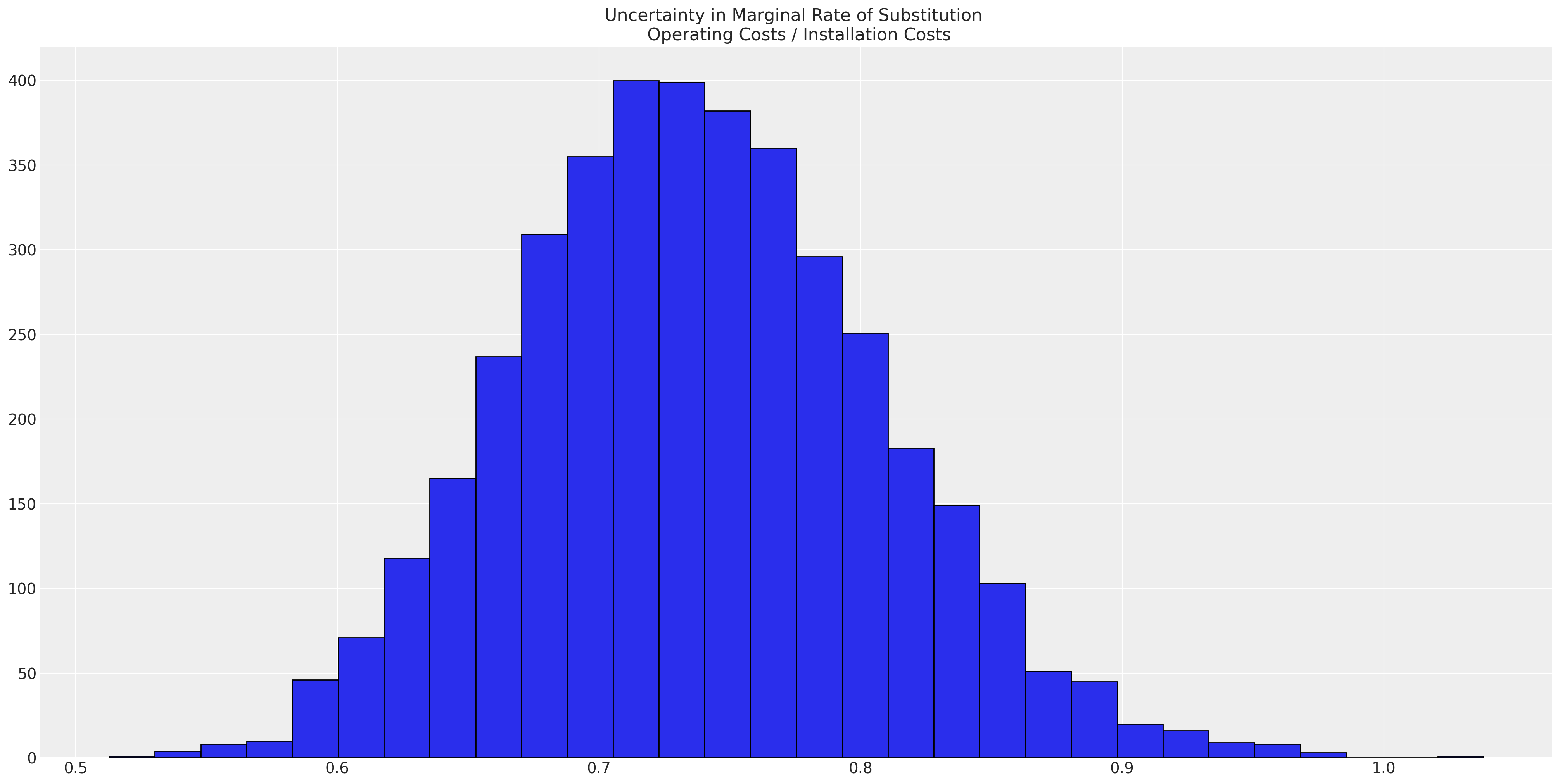
这表明,相对于一次性安装成本而言,经常性运营成本每单位减少的价值约为 0.7。这是否在遥远的程度上是合理的几乎无关紧要,因为该模型甚至没有密切捕捉到数据生成过程。但值得重申的是,效用的原始尺度并非直接有意义,但效用方程中系数的比率可以直接解释。
为了评估模型的总体充分性,我们可以依靠后验预测检查来查看模型是否可以恢复数据生成过程的近似值。
idata_m1["posterior"]["p"].mean(dim=["chain", "draw", "obs"])
<xarray.DataArray 'p' (alts_probs: 5)>
array([0.10421251, 0.05138074, 0.51701653, 0.24023285, 0.08715736])
Coordinates:
  * alts_probs  (alts_probs) <U2 'ec' 'er' 'gc' 'gr' 'hp'
fig, axs = plt.subplots(1, 2, figsize=(20, 10))
ax = axs[0]
counts = wide_heating_df.groupby("depvar")["idcase"].count()
predicted_shares = idata_m1["posterior"]["p"].mean(dim=["chain", "draw", "obs"])
ci_lb = idata_m1["posterior"]["p"].quantile(0.025, dim=["chain", "draw", "obs"])
ci_ub = idata_m1["posterior"]["p"].quantile(0.975, dim=["chain", "draw", "obs"])
ax.scatter(ci_lb, ["ec", "er", "gc", "gr", "hp"], color="k", s=2)
ax.scatter(ci_ub, ["ec", "er", "gc", "gr", "hp"], color="k", s=2)
ax.scatter(
    counts / counts.sum(),
    ["ec", "er", "gc", "gr", "hp"],
    label="Observed Shares",
    color="red",
    s=100,
)
ax.hlines(
    ["ec", "er", "gc", "gr", "hp"], ci_lb, ci_ub, label="Predicted 95% Interval", color="black"
)
ax.legend()
ax.set_title("Observed V Predicted Shares")
az.plot_ppc(idata_m1, ax=axs[1])
axs[1].set_title("Posterior Predictive Checks")
ax.set_xlabel("Shares")
ax.set_ylabel("Heating System");
/Users/nathanielforde/mambaforge/envs/pymc_examples_new/lib/python3.9/site-packages/arviz/plots/ppcplot.py:267: FutureWarning: The return type of `Dataset.dims` will be changed to return a set of dimension names in future, in order to be more consistent with `DataArray.dims`. To access a mapping from dimension names to lengths, please use `Dataset.sizes`.
  flatten_pp = list(predictive_dataset.dims.keys())
/Users/nathanielforde/mambaforge/envs/pymc_examples_new/lib/python3.9/site-packages/arviz/plots/ppcplot.py:271: FutureWarning: The return type of `Dataset.dims` will be changed to return a set of dimension names in future, in order to be more consistent with `DataArray.dims`. To access a mapping from dimension names to lengths, please use `Dataset.sizes`.
  flatten = list(observed_data.dims.keys())
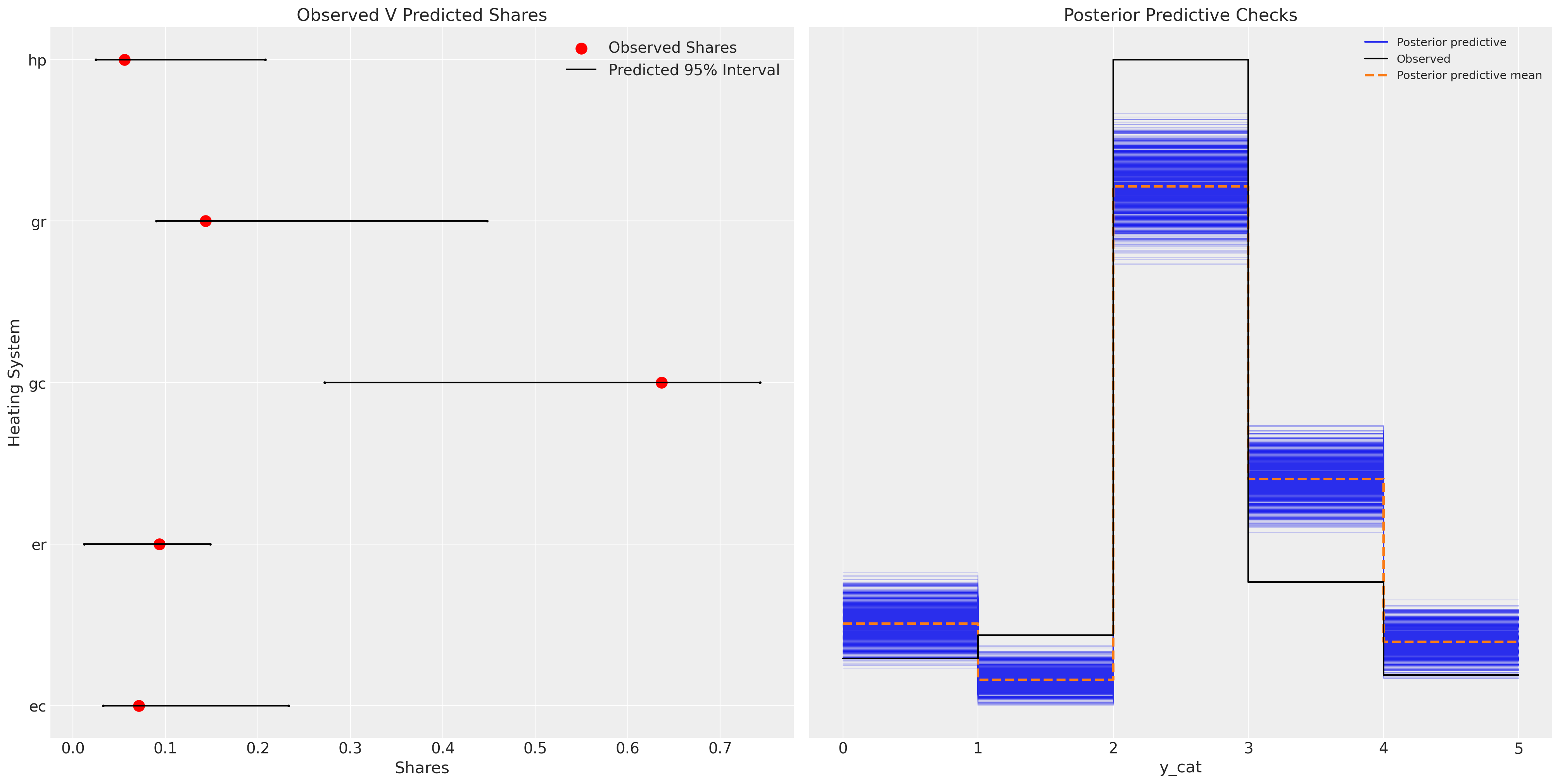
我们可以在这里看到,该模型相当不充分,并且在重新捕获后验预测分布方面非常失败。
改进的模型:添加备选方案特定截距#
我们可以通过为每个独特的备选方案 gr, gc, ec, er 添加截距项来解决先前模型规范中的一些问题。这些项将通过允许我们控制跨产品效用度量的一些异质性来吸收上一个模型中看到的一些误差。
N = wide_heating_df.shape[0]
observed = pd.Categorical(wide_heating_df["depvar"]).codes

coords = {
    "alts_intercepts": ["ec", "er", "gc", "gr"],
    "alts_probs": ["ec", "er", "gc", "gr", "hp"],
    "obs": range(N),
}
with pm.Model(coords=coords) as model_2:
    beta_ic = pm.Normal("beta_ic", 0, 1)
    beta_oc = pm.Normal("beta_oc", 0, 1)
    alphas = pm.Normal("alpha", 0, 1, dims="alts_intercepts")

    ## Construct Utility matrix and Pivot using an intercept per alternative
    u0 = alphas[0] + beta_ic * wide_heating_df["ic.ec"] + beta_oc * wide_heating_df["oc.ec"]
    u1 = alphas[1] + beta_ic * wide_heating_df["ic.er"] + beta_oc * wide_heating_df["oc.er"]
    u2 = alphas[2] + beta_ic * wide_heating_df["ic.gc"] + beta_oc * wide_heating_df["oc.gc"]
    u3 = alphas[3] + beta_ic * wide_heating_df["ic.gr"] + beta_oc * wide_heating_df["oc.gr"]
    u4 = 0 + beta_ic * wide_heating_df["ic.hp"] + beta_oc * wide_heating_df["oc.hp"]
    s = pm.math.stack([u0, u1, u2, u3, u4]).T

    ## Apply Softmax Transform
    p_ = pm.Deterministic("p", pm.math.softmax(s, axis=1), dims=("obs", "alts_probs"))

    ## Likelihood
    choice_obs = pm.Categorical("y_cat", p=p_, observed=observed, dims="obs")

    idata_m2 = pm.sample_prior_predictive()
    idata_m2.extend(
        pm.sample(nuts_sampler="numpyro", idata_kwargs={"log_likelihood": True}, random_seed=103)
    )
    idata_m2.extend(pm.sample_posterior_predictive(idata_m2))


pm.model_to_graphviz(model_2)
Sampling: [alpha, beta_ic, beta_oc, y_cat]
/Users/nathanielforde/mambaforge/envs/pymc_examples_new/lib/python3.9/site-packages/pymc/sampling/mcmc.py:243: UserWarning: Use of external NUTS sampler is still experimental
  warnings.warn("Use of external NUTS sampler is still experimental", UserWarning)
Compiling...
Compilation time =  0:00:01.074196
Sampling...
Sampling time =  0:00:12.000761
Transforming variables...
Transformation time =  0:00:00.295025
Computing Log Likelihood...
Sampling: [y_cat]
Log Likelihood time = 0:00:00.411164

我们有意将 hp 备选方案的截距参数归零,以确保参数识别是可行的。
az.summary(idata_m2, var_names=["beta_ic", "beta_oc", "alpha"], round_to=4)
| 平均值 | 标准差 | hdi_3% | hdi_97% | mcse_mean | mcse_sd | ess_bulk | ess_tail | r_hat | |
|---|---|---|---|---|---|---|---|---|---|
| beta_ic | -0.0019 | 0.0006 | -0.0030 | -0.0007 | 0.0000 | 0.0000 | 2194.2030 | 2974.0194 | 1.0004 |
| beta_oc | -0.0058 | 0.0013 | -0.0082 | -0.0032 | 0.0000 | 0.0000 | 1317.1605 | 1482.4796 | 1.0008 |
| alpha[ec] | 1.1859 | 0.3856 | 0.4164 | 1.8939 | 0.0111 | 0.0079 | 1208.3253 | 1521.0849 | 1.0009 |
| alpha[er] | 1.4859 | 0.3102 | 0.8716 | 2.0489 | 0.0088 | 0.0063 | 1244.2319 | 1021.4642 | 1.0009 |
| alpha[gc] | 1.6028 | 0.2169 | 1.1950 | 2.0159 | 0.0060 | 0.0043 | 1319.9286 | 1489.0237 | 1.0011 |
| alpha[gr] | 0.2644 | 0.1925 | -0.0933 | 0.6262 | 0.0051 | 0.0037 | 1408.3095 | 1595.1160 | 1.0011 |
我们现在可以看到此模型在捕获数据生成过程的各个方面方面表现得更好。
fig, axs = plt.subplots(1, 2, figsize=(20, 10))
ax = axs[0]
counts = wide_heating_df.groupby("depvar")["idcase"].count()
predicted_shares = idata_m2["posterior"]["p"].mean(dim=["chain", "draw", "obs"])
ci_lb = idata_m2["posterior"]["p"].quantile(0.025, dim=["chain", "draw", "obs"])
ci_ub = idata_m2["posterior"]["p"].quantile(0.975, dim=["chain", "draw", "obs"])

ax.scatter(ci_lb, ["ec", "er", "gc", "gr", "hp"], color="k", s=2)
ax.scatter(ci_ub, ["ec", "er", "gc", "gr", "hp"], color="k", s=2)
ax.scatter(
    counts / counts.sum(),
    ["ec", "er", "gc", "gr", "hp"],
    label="Observed Shares",
    color="red",
    s=100,
)
ax.hlines(
    ["ec", "er", "gc", "gr", "hp"], ci_lb, ci_ub, label="Predicted 95% Interval", color="black"
)
ax.legend()
ax.set_title("Observed V Predicted Shares")
az.plot_ppc(idata_m2, ax=axs[1])
axs[1].set_title("Posterior Predictive Checks")
ax.set_xlabel("Shares")
ax.set_ylabel("Heating System");
/Users/nathanielforde/mambaforge/envs/pymc_examples_new/lib/python3.9/site-packages/arviz/plots/ppcplot.py:267: FutureWarning: The return type of `Dataset.dims` will be changed to return a set of dimension names in future, in order to be more consistent with `DataArray.dims`. To access a mapping from dimension names to lengths, please use `Dataset.sizes`.
  flatten_pp = list(predictive_dataset.dims.keys())
/Users/nathanielforde/mambaforge/envs/pymc_examples_new/lib/python3.9/site-packages/arviz/plots/ppcplot.py:271: FutureWarning: The return type of `Dataset.dims` will be changed to return a set of dimension names in future, in order to be more consistent with `DataArray.dims`. To access a mapping from dimension names to lengths, please use `Dataset.sizes`.
  flatten = list(observed_data.dims.keys())
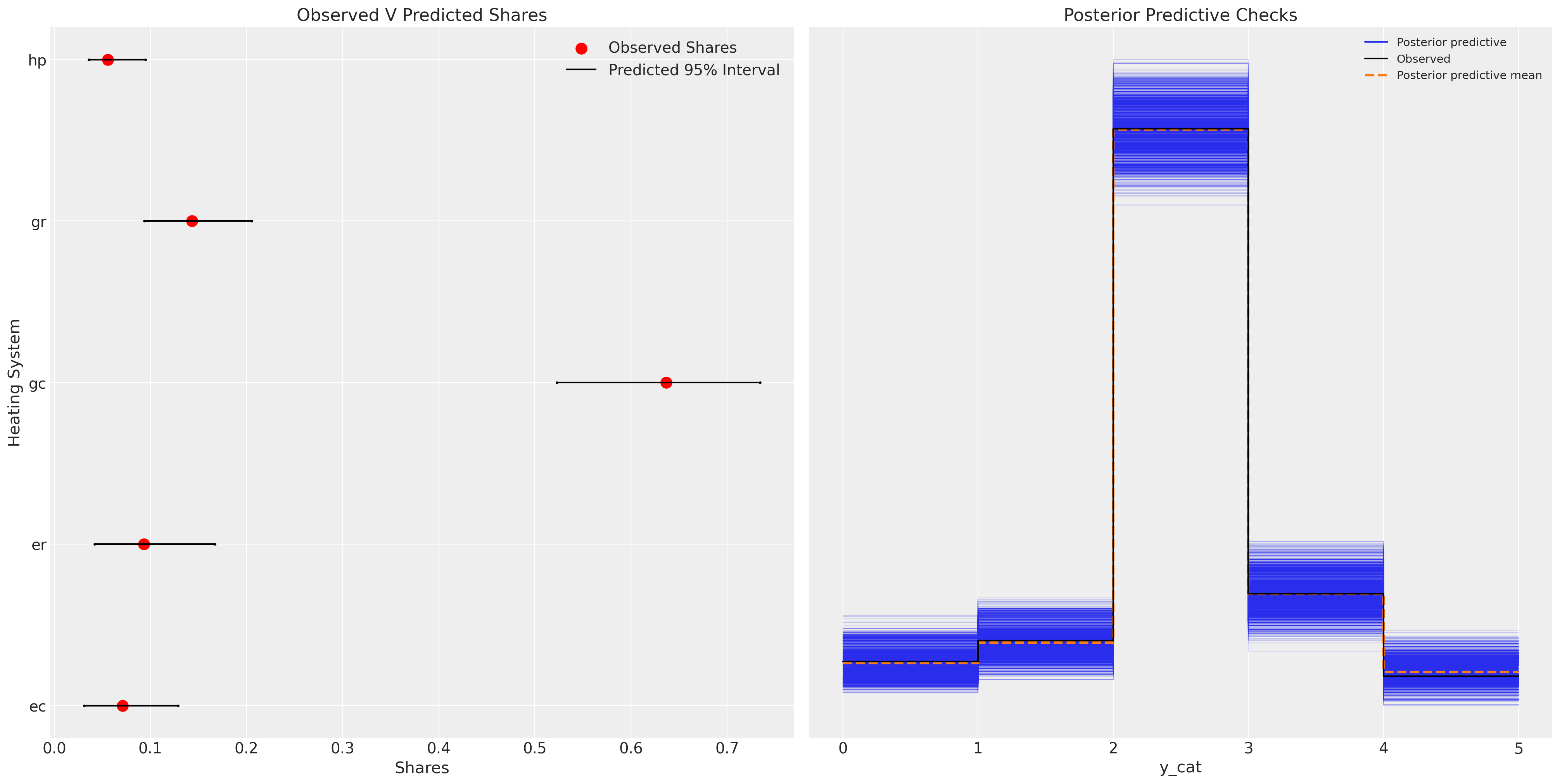
此模型代表了实质性的改进。
实验模型:添加相关结构#
我们可能会认为备选商品之间存在相关性,我们也应该捕捉到这种相关性。我们可以通过在截距(或备选地,beta 参数)上放置多元正态先验来捕捉这些效应(如果它们存在)。此外,我们还添加了关于收入影响每个备选方案效用的信息。
coords = {
    "alts_intercepts": ["ec", "er", "gc", "gr"],
    "alts_probs": ["ec", "er", "gc", "gr", "hp"],
    "obs": range(N),
}
with pm.Model(coords=coords) as model_3:
    ## Add data to experiment with changes later.
    ic_ec = pm.MutableData("ic_ec", wide_heating_df["ic.ec"])
    oc_ec = pm.MutableData("oc_ec", wide_heating_df["oc.ec"])
    ic_er = pm.MutableData("ic_er", wide_heating_df["ic.er"])
    oc_er = pm.MutableData("oc_er", wide_heating_df["oc.er"])

    beta_ic = pm.Normal("beta_ic", 0, 1)
    beta_oc = pm.Normal("beta_oc", 0, 1)
    chol, corr, stds = pm.LKJCholeskyCov(
        "chol", n=5, eta=2.0, sd_dist=pm.Exponential.dist(1.0, shape=5)
    )
    alphas = pm.MvNormal("alpha", mu=0, chol=chol, dims="alts_probs")

    u0 = alphas[0] + beta_ic * ic_ec + beta_oc * oc_ec
    u1 = alphas[1] + beta_ic * ic_er + beta_oc * oc_er
    u2 = alphas[2] + beta_ic * wide_heating_df["ic.gc"] + beta_oc * wide_heating_df["oc.gc"]
    u3 = alphas[3] + beta_ic * wide_heating_df["ic.gr"] + beta_oc * wide_heating_df["oc.gr"]
    u4 = (
        alphas[4] + beta_ic * wide_heating_df["ic.hp"] + beta_oc * wide_heating_df["oc.hp"]
    )  # pivot)
    s = pm.math.stack([u0, u1, u2, u3, u4]).T

    p_ = pm.Deterministic("p", pm.math.softmax(s, axis=1), dims=("obs", "alts_probs"))
    choice_obs = pm.Categorical("y_cat", p=p_, observed=observed, dims="obs")

    idata_m3 = pm.sample_prior_predictive()
    idata_m3.extend(
        pm.sample(nuts_sampler="numpyro", idata_kwargs={"log_likelihood": True}, random_seed=100)
    )
    idata_m3.extend(pm.sample_posterior_predictive(idata_m3))


pm.model_to_graphviz(model_3)
Sampling: [alpha, beta_ic, beta_oc, chol, y_cat]
/Users/nathanielforde/mambaforge/envs/pymc_examples_new/lib/python3.9/site-packages/pymc/sampling/mcmc.py:243: UserWarning: Use of external NUTS sampler is still experimental
  warnings.warn("Use of external NUTS sampler is still experimental", UserWarning)
Compiling...
Compilation time =  0:00:02.342931
Sampling...
Sampling time =  0:00:23.358412
Transforming variables...
Transformation time =  0:00:00.553256
Computing Log Likelihood...
Sampling: [y_cat]
Log Likelihood time = 0:00:00.446564

绘制模型拟合图,我们看到了类似的故事。模型预测性能没有显着提高,并且我们为模型增加了一些复杂性。这种额外的复杂性应该在诸如 AIC 和 WAIC 之类的模型评估指标中受到惩罚。但通常,产品之间的相关性是一些感兴趣的特征,与历史预测问题无关。
fig, axs = plt.subplots(1, 2, figsize=(20, 10))
ax = axs[0]
counts = wide_heating_df.groupby("depvar")["idcase"].count()
predicted_shares = idata_m3["posterior"]["p"].mean(dim=["chain", "draw", "obs"])
ci_lb = idata_m3["posterior"]["p"].quantile(0.025, dim=["chain", "draw", "obs"])
ci_ub = idata_m3["posterior"]["p"].quantile(0.975, dim=["chain", "draw", "obs"])

ax.scatter(ci_lb, ["ec", "er", "gc", "gr", "hp"], color="k", s=2)
ax.scatter(ci_ub, ["ec", "er", "gc", "gr", "hp"], color="k", s=2)
ax.scatter(
    counts / counts.sum(),
    ["ec", "er", "gc", "gr", "hp"],
    label="Observed Shares",
    color="red",
    s=100,
)
ax.hlines(
    ["ec", "er", "gc", "gr", "hp"], ci_lb, ci_ub, label="Predicted 95% Interval", color="black"
)
ax.legend()
ax.set_title("Observed V Predicted Shares")
az.plot_ppc(idata_m3, ax=axs[1])
axs[1].set_title("Posterior Predictive Checks")
ax.set_xlabel("Shares")
ax.set_ylabel("Heating System");
/Users/nathanielforde/mambaforge/envs/pymc_examples_new/lib/python3.9/site-packages/arviz/plots/ppcplot.py:267: FutureWarning: The return type of `Dataset.dims` will be changed to return a set of dimension names in future, in order to be more consistent with `DataArray.dims`. To access a mapping from dimension names to lengths, please use `Dataset.sizes`.
  flatten_pp = list(predictive_dataset.dims.keys())
/Users/nathanielforde/mambaforge/envs/pymc_examples_new/lib/python3.9/site-packages/arviz/plots/ppcplot.py:271: FutureWarning: The return type of `Dataset.dims` will be changed to return a set of dimension names in future, in order to be more consistent with `DataArray.dims`. To access a mapping from dimension names to lengths, please use `Dataset.sizes`.
  flatten = list(observed_data.dims.keys())
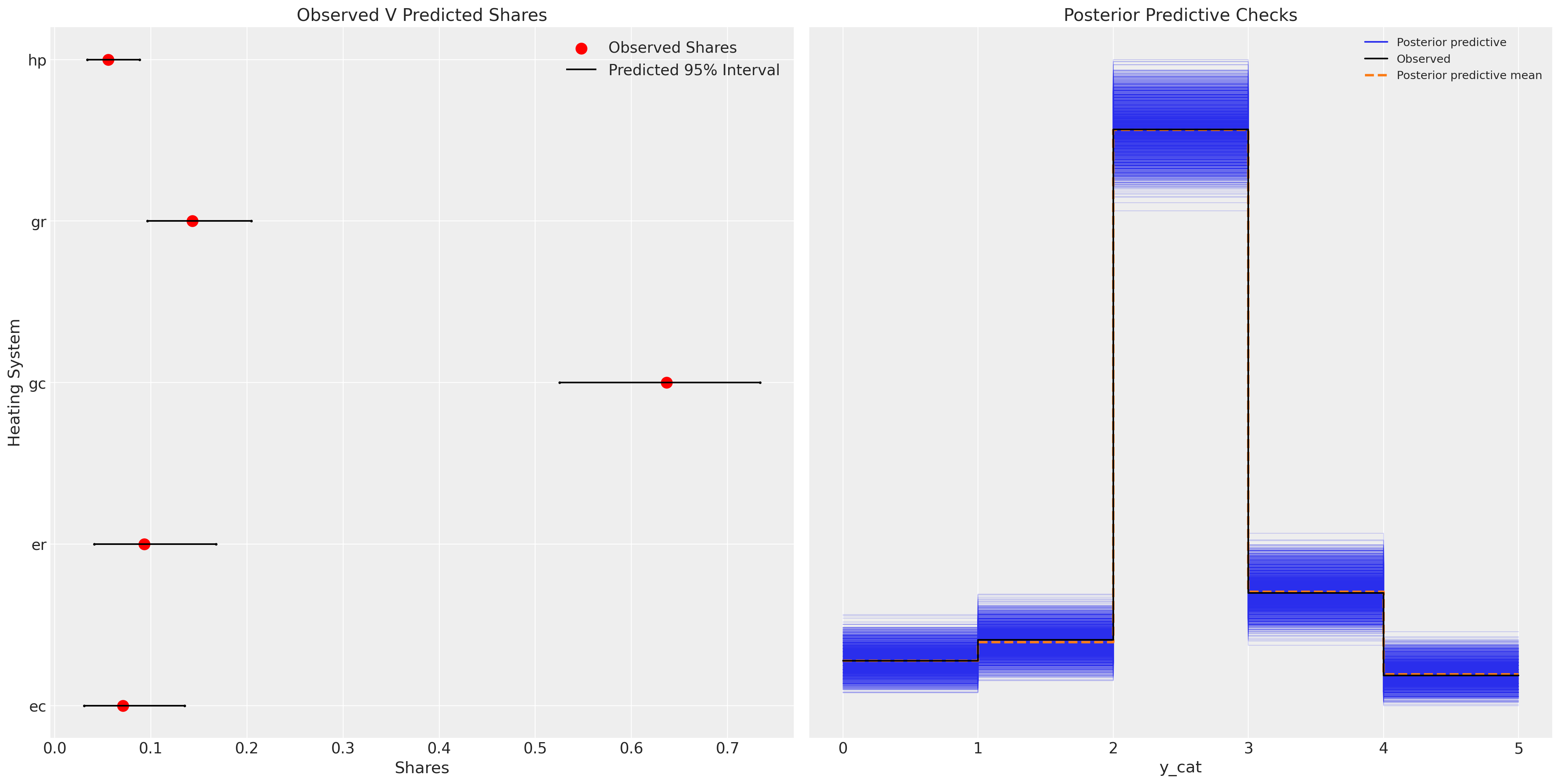
额外的复杂性可能提供信息,并且备选产品之间的关系程度将告知政策变化下的替代模式。另请注意,在此模型规范下,beta_ic 的参数的期望值为 0。这可能暗示着对安装成本现实的无奈接受,这种接受在决定购买后不会以任何方式改变效用度量。
az.summary(idata_m3, var_names=["beta_ic", "beta_oc", "alpha", "chol_corr"], round_to=4)
/Users/nathanielforde/mambaforge/envs/pymc_examples_new/lib/python3.9/site-packages/arviz/stats/diagnostics.py:592: RuntimeWarning: invalid value encountered in scalar divide
  (between_chain_variance / within_chain_variance + num_samples - 1) / (num_samples)
| 平均值 | 标准差 | hdi_3% | hdi_97% | mcse_mean | mcse_sd | ess_bulk | ess_tail | r_hat | |
|---|---|---|---|---|---|---|---|---|---|
| beta_ic | -0.0016 | 0.0006 | -0.0028 | -0.0005 | 0.0000 | 0.0000 | 965.4150 | 1858.7119 | 1.0001 |
| beta_oc | -0.0063 | 0.0014 | -0.0088 | -0.0035 | 0.0001 | 0.0001 | 279.5321 | 415.1640 | 1.0173 |
| alpha[ec] | 0.1390 | 0.4889 | -0.6647 | 1.2387 | 0.0379 | 0.0268 | 231.0307 | 299.2109 | 1.0194 |
| alpha[er] | 0.3534 | 0.5002 | -0.2853 | 1.5779 | 0.0414 | 0.0293 | 194.8276 | 248.4286 | 1.0183 |
| alpha[gc] | 0.3954 | 0.5681 | -0.3446 | 1.5776 | 0.0532 | 0.0380 | 112.9666 | 358.4609 | 1.0290 |
| alpha[gr] | -0.9796 | 0.5950 | -1.8111 | 0.1638 | 0.0579 | 0.0410 | 105.7955 | 427.4041 | 1.0316 |
| alpha[hp] | -1.3157 | 0.5856 | -2.1852 | -0.1067 | 0.0539 | 0.0382 | 141.3095 | 215.2878 | 1.0236 |
| chol_corr[0, 0] | 1.0000 | 0.0000 | 1.0000 | 1.0000 | 0.0000 | 0.0000 | 4000.0000 | 4000.0000 | NaN |
| chol_corr[0, 1] | 0.0324 | 0.3416 | -0.5952 | 0.6568 | 0.0087 | 0.0077 | 1546.9802 | 1197.8477 | 1.0018 |
| chol_corr[0, 2] | 0.0061 | 0.3520 | -0.6189 | 0.6374 | 0.0157 | 0.0111 | 825.6169 | 1945.6811 | 1.0142 |
| chol_corr[0, 3] | 0.0092 | 0.3332 | -0.5888 | 0.6468 | 0.0077 | 0.0069 | 1890.5246 | 1531.3933 | 1.0180 |
| chol_corr[0, 4] | 0.0476 | 0.3611 | -0.6530 | 0.5964 | 0.0439 | 0.0312 | 69.4621 | 1858.2409 | 1.0408 |
| chol_corr[1, 0] | 0.0324 | 0.3416 | -0.5952 | 0.6568 | 0.0087 | 0.0077 | 1546.9802 | 1197.8477 | 1.0018 |
| chol_corr[1, 1] | 1.0000 | 0.0000 | 1.0000 | 1.0000 | 0.0000 | 0.0000 | 1802.6889 | 1658.0984 | 1.0002 |
| chol_corr[1, 2] | 0.0341 | 0.3451 | -0.5745 | 0.6690 | 0.0180 | 0.0127 | 440.1281 | 2672.0734 | 1.0144 |
| chol_corr[1, 3] | -0.0490 | 0.3437 | -0.6373 | 0.6208 | 0.0118 | 0.0084 | 1201.2989 | 1567.5346 | 1.0077 |
| chol_corr[1, 4] | -0.0750 | 0.3409 | -0.6803 | 0.5525 | 0.0106 | 0.0075 | 1284.5413 | 1900.4899 | 1.0091 |
| chol_corr[2, 0] | 0.0061 | 0.3520 | -0.6189 | 0.6374 | 0.0157 | 0.0111 | 825.6169 | 1945.6811 | 1.0142 |
| chol_corr[2, 1] | 0.0341 | 0.3451 | -0.5745 | 0.6690 | 0.0180 | 0.0127 | 440.1281 | 2672.0734 | 1.0144 |
| chol_corr[2, 2] | 1.0000 | 0.0000 | 1.0000 | 1.0000 | 0.0000 | 0.0000 | 2150.3579 | 3042.5649 | 1.0008 |
| chol_corr[2, 3] | -0.0517 | 0.3398 | -0.6596 | 0.5873 | 0.0163 | 0.0115 | 515.9573 | 2505.1328 | 1.0134 |
| chol_corr[2, 4] | -0.0264 | 0.3375 | -0.6438 | 0.5736 | 0.0174 | 0.0123 | 456.2480 | 2197.2798 | 1.0154 |
| chol_corr[3, 0] | 0.0092 | 0.3332 | -0.5888 | 0.6468 | 0.0077 | 0.0069 | 1890.5246 | 1531.3933 | 1.0180 |
| chol_corr[3, 1] | -0.0490 | 0.3437 | -0.6373 | 0.6208 | 0.0118 | 0.0084 | 1201.2989 | 1567.5346 | 1.0077 |
| chol_corr[3, 2] | -0.0517 | 0.3398 | -0.6596 | 0.5873 | 0.0163 | 0.0115 | 515.9573 | 2505.1328 | 1.0134 |
| chol_corr[3, 3] | 1.0000 | 0.0000 | 1.0000 | 1.0000 | 0.0000 | 0.0000 | 3216.9877 | 3379.4979 | 1.0047 |
| chol_corr[3, 4] | 0.1003 | 0.3591 | -0.4994 | 0.7509 | 0.0573 | 0.0408 | 43.4352 | 336.8334 | 1.0650 |
| chol_corr[4, 0] | 0.0476 | 0.3611 | -0.6530 | 0.5964 | 0.0439 | 0.0312 | 69.4621 | 1858.2409 | 1.0408 |
| chol_corr[4, 1] | -0.0750 | 0.3409 | -0.6803 | 0.5525 | 0.0106 | 0.0075 | 1284.5413 | 1900.4899 | 1.0091 |
| chol_corr[4, 2] | -0.0264 | 0.3375 | -0.6438 | 0.5736 | 0.0174 | 0.0123 | 456.2480 | 2197.2798 | 1.0154 |
| chol_corr[4, 3] | 0.1003 | 0.3591 | -0.4994 | 0.7509 | 0.0573 | 0.0408 | 43.4352 | 336.8334 | 1.0650 |
| chol_corr[4, 4] | 1.0000 | 0.0000 | 1.0000 | 1.0000 | 0.0000 | 0.0000 | 1901.4003 | 2561.2466 | 1.0022 |
在此模型中,我们看到边际替代率表明,运营成本增加一美元对效用计算的影响几乎是安装成本类似增加的 17 倍。这在某种程度上是有道理的,因为我们可以预期安装成本是一次性支出,我们对此非常无奈。
post = az.extract(idata_m3)
substitution_rate = post["beta_oc"] / post["beta_ic"]
substitution_rate.mean().item()
4.312409953314165
市场干预和预测市场份额#
我们还可以使用这些类型的模型来预测价格干预下的市场份额变化。
with model_3:
    # update values of predictors with new 20% price increase in operating costs for electrical options
    pm.set_data({"oc_ec": wide_heating_df["oc.ec"] * 1.2, "oc_er": wide_heating_df["oc.er"] * 1.2})
    # use the updated values and predict outcomes and probabilities:
    idata_new_policy = pm.sample_posterior_predictive(
        idata_m3,
        var_names=["p", "y_cat"],
        return_inferencedata=True,
        predictions=True,
        extend_inferencedata=False,
        random_seed=100,
    )

idata_new_policy
Sampling: [y_cat]
-
<xarray.Dataset> Dimensions: (chain: 4, draw: 1000, obs: 900, alts_probs: 5) Coordinates: * chain (chain) int64 0 1 2 3 * draw (draw) int64 0 1 2 3 4 5 6 7 ... 992 993 994 995 996 997 998 999 * obs (obs) int64 0 1 2 3 4 5 6 7 ... 892 893 894 895 896 897 898 899 * alts_probs (alts_probs) <U2 'ec' 'er' 'gc' 'gr' 'hp' Data variables: p (chain, draw, obs, alts_probs) float64 0.03931 ... 0.05623 y_cat (chain, draw, obs) int64 2 4 4 2 1 2 2 2 2 ... 2 4 3 3 2 2 2 4 2 Attributes: created_at: 2025-03-22T20:11:54.000714 arviz_version: 0.17.0 inference_library: pymc inference_library_version: 5.3.0 -
<xarray.Dataset>
Dimensions:      (ic_ec_dim_0: 900, oc_ec_dim_0: 900, ic_er_dim_0: 900,
                  oc_er_dim_0: 900)
Coordinates:
  * ic_ec_dim_0  (ic_ec_dim_0) int64 0 1 2 3 4 5 6 ... 894 895 896 897 898 899
  * oc_ec_dim_0  (oc_ec_dim_0) int64 0 1 2 3 4 5 6 ... 894 895 896 897 898 899
  * ic_er_dim_0  (ic_er_dim_0) int64 0 1 2 3 4 5 6 ... 894 895 896 897 898 899
  * oc_er_dim_0  (oc_er_dim_0) int64 0 1 2 3 4 5 6 ... 894 895 896 897 898 899
Data variables:
    ic_ec        (ic_ec_dim_0) float64 859.9 796.8 719.9 ... 842.8 799.8 967.9
    oc_ec        (oc_ec_dim_0) float64 664.0 624.3 526.9 ... 574.6 594.2 622.4
    ic_er        (ic_er_dim_0) float64 995.8 894.7 900.1 ... 1.123e+03 1.092e+03
    oc_er        (oc_er_dim_0) float64 606.7 583.8 485.7 ... 538.3 481.9 550.2
Attributes:
    created_at:                 2025-03-22T20:11:54.004944
    arviz_version:              0.17.0
    inference_library:          pymc
    inference_library_version:  5.3.0
# Old Policy Expectations
old = idata_m3["posterior"]["p"].mean(dim=["chain", "draw", "obs"])
old
<xarray.DataArray 'p' (alts_probs: 5)>
array([0.07133772, 0.09128577, 0.63642949, 0.14428672, 0.05666029])
Coordinates:
  * alts_probs  (alts_probs) <U2 'ec' 'er' 'gc' 'gr' 'hp'
# New Policy Expectations
new = idata_new_policy["predictions"]["p"].mean(dim=["chain", "draw", "obs"])
new
<xarray.DataArray 'p' (alts_probs: 5)>
array([0.04381375, 0.05912996, 0.68165693, 0.15463743, 0.06076193])
Coordinates:
  * alts_probs  (alts_probs) <U2 'ec' 'er' 'gc' 'gr' 'hp'
new - old
<xarray.DataArray 'p' (alts_probs: 5)>
array([-0.02752397, -0.03215581,  0.04522743,  0.01035071,  0.00410164])
Coordinates:
  * alts_probs  (alts_probs) <U2 'ec' 'er' 'gc' 'gr' 'hp'
fig, ax = plt.subplots(1, figsize=(20, 10))
counts = wide_heating_df.groupby("depvar")["idcase"].count()
new_predictions = idata_new_policy["predictions"]["p"].mean(dim=["chain", "draw", "obs"]).values
ci_lb = idata_m3["posterior"]["p"].quantile(0.025, dim=["chain", "draw", "obs"])
ci_ub = idata_m3["posterior"]["p"].quantile(0.975, dim=["chain", "draw", "obs"])
ax.scatter(ci_lb, ["ec", "er", "gc", "gr", "hp"], color="k", s=2)
ax.scatter(ci_ub, ["ec", "er", "gc", "gr", "hp"], color="k", s=2)
ax.scatter(
    new_predictions,
    ["ec", "er", "gc", "gr", "hp"],
    color="green",
    label="New Policy Predicted Share",
    s=100,
)
ax.scatter(
    counts / counts.sum(),
    ["ec", "er", "gc", "gr", "hp"],
    label="Observed Shares",
    color="red",
    s=100,
)
ax.hlines(
    ["ec", "er", "gc", "gr", "hp"],
    ci_lb,
    ci_ub,
    label="Predicted 95% Credible Interval Old Policy",
    color="black",
)
ax.set_title("Predicted Market Shares under Old and New Pricing Policy", fontsize=20)
ax.set_xlabel("Market Share")
ax.legend();
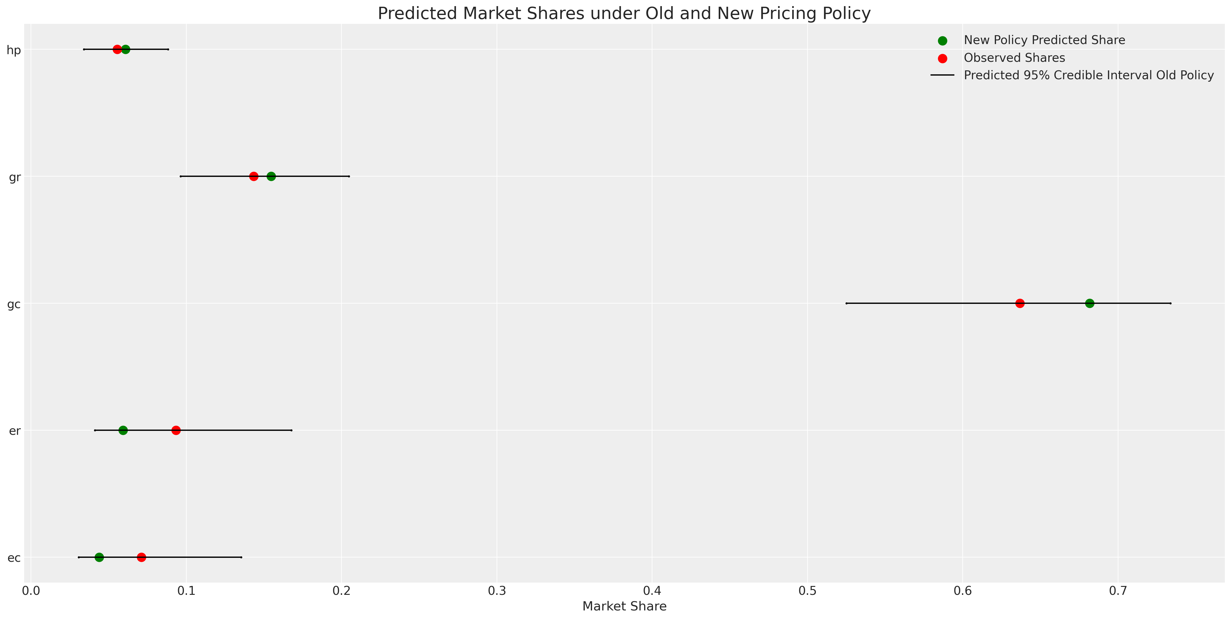
在这里,我们可以看到,正如预期的那样,电力选项的运营成本上升对其预测的市场份额产生了负面影响。
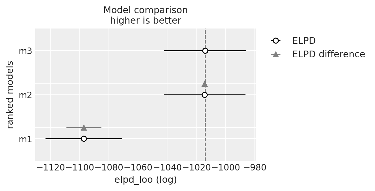
比较模型#
我们现在将评估所有三个模型拟合的预测性能。原始数据的预测性能是一个很好的基准,表明该模型已适当地捕获了数据生成过程。但正如我们所见,这并不是这些模型中唯一感兴趣的特征。这些模型对我们对做出决策的代理人、决策过程的观点以及选择场景的要素的理论信念很敏感。
compare = az.compare({"m1": idata_m1, "m2": idata_m2, "m3": idata_m3})
compare
| rank | elpd_loo | p_loo | elpd_diff | weight | se | dse | warning | scale | |
|---|---|---|---|---|---|---|---|---|---|
| m3 | 0 | -1014.070339 | 5.636640 | 0.000000 | 1.000000e+00 | 27.994286 | 0.000000 | False | log |
| m2 | 1 | -1014.343946 | 5.398733 | 0.273607 | 1.067993e-10 | 27.880217 | 0.733146 | False | log |
| m1 | 2 | -1097.230815 | 1.999354 | 83.160476 | 0.000000e+00 | 26.259507 | 12.010909 | False | log |
az.plot_compare(compare);
在重复选择中选择饼干:混合 Logit 模型#
转到另一个示例,我们看到了一个选择场景,其中对同一个人就其在备选方案中选择饼干的情况进行了多次民意调查。这为我们提供了通过为每个产品的个人添加系数来评估个人偏好的机会。
try:
    c_df = pd.read_csv("../data/cracker_choice_short.csv")
except:
    c_df = pd.read_csv(pm.get_data("cracker_choice_short.csv"))
columns = [c for c in c_df.columns if c != "Unnamed: 0"]
c_df[columns]
| personId | disp.sunshine | disp.keebler | disp.nabisco | disp.private | feat.sunshine | feat.keebler | feat.nabisco | feat.private | price.sunshine | price.keebler | price.nabisco | price.private | choice | lastChoice | personChoiceId | choiceId | |
|---|---|---|---|---|---|---|---|---|---|---|---|---|---|---|---|---|---|
| 0 | 1 | 0 | 0 | 0 | 0 | 0 | 0 | 0 | 0 | 0.99 | 1.09 | 0.99 | 0.71 | nabisco | nabisco | 1 | 1 |
| 1 | 1 | 1 | 0 | 0 | 0 | 0 | 0 | 0 | 0 | 0.49 | 1.09 | 1.09 | 0.78 | sunshine | nabisco | 2 | 2 |
| 2 | 1 | 0 | 0 | 0 | 0 | 0 | 0 | 0 | 0 | 1.03 | 1.09 | 0.89 | 0.78 | nabisco | sunshine | 3 | 3 |
| 3 | 1 | 0 | 0 | 0 | 0 | 0 | 0 | 0 | 0 | 1.09 | 1.09 | 1.19 | 0.64 | nabisco | nabisco | 4 | 4 |
| 4 | 1 | 0 | 0 | 0 | 0 | 0 | 0 | 0 | 0 | 0.89 | 1.09 | 1.19 | 0.84 | nabisco | nabisco | 5 | 5 |
| ... | ... | ... | ... | ... | ... | ... | ... | ... | ... | ... | ... | ... | ... | ... | ... | ... | ... |
| 3151 | 136 | 0 | 0 | 0 | 0 | 0 | 0 | 0 | 0 | 1.09 | 1.19 | 0.99 | 0.55 | private | private | 9 | 3152 |
| 3152 | 136 | 0 | 0 | 0 | 1 | 0 | 0 | 0 | 0 | 0.78 | 1.35 | 1.04 | 0.65 | private | private | 10 | 3153 |
| 3153 | 136 | 0 | 0 | 0 | 0 | 0 | 0 | 0 | 0 | 1.09 | 1.17 | 1.29 | 0.59 | private | private | 11 | 3154 |
| 3154 | 136 | 0 | 0 | 0 | 0 | 0 | 0 | 0 | 0 | 1.09 | 1.22 | 1.29 | 0.59 | private | private | 12 | 3155 |
| 3155 | 136 | 0 | 0 | 0 | 0 | 0 | 0 | 0 | 0 | 1.29 | 1.04 | 1.23 | 0.59 | private | private | 13 | 3156 |
3156 行 × 17 列
c_df.groupby("personId")[["choiceId"]].count().T
| personId | 1 | 2 | 3 | 4 | 5 | 6 | 7 | 8 | 9 | 10 | ... | 127 | 128 | 129 | 130 | 131 | 132 | 133 | 134 | 135 | 136 |
|---|---|---|---|---|---|---|---|---|---|---|---|---|---|---|---|---|---|---|---|---|---|
| choiceId | 15 | 15 | 13 | 28 | 13 | 27 | 16 | 25 | 18 | 40 | ... | 17 | 25 | 31 | 31 | 29 | 21 | 26 | 13 | 14 | 13 |
1 行 × 136 列
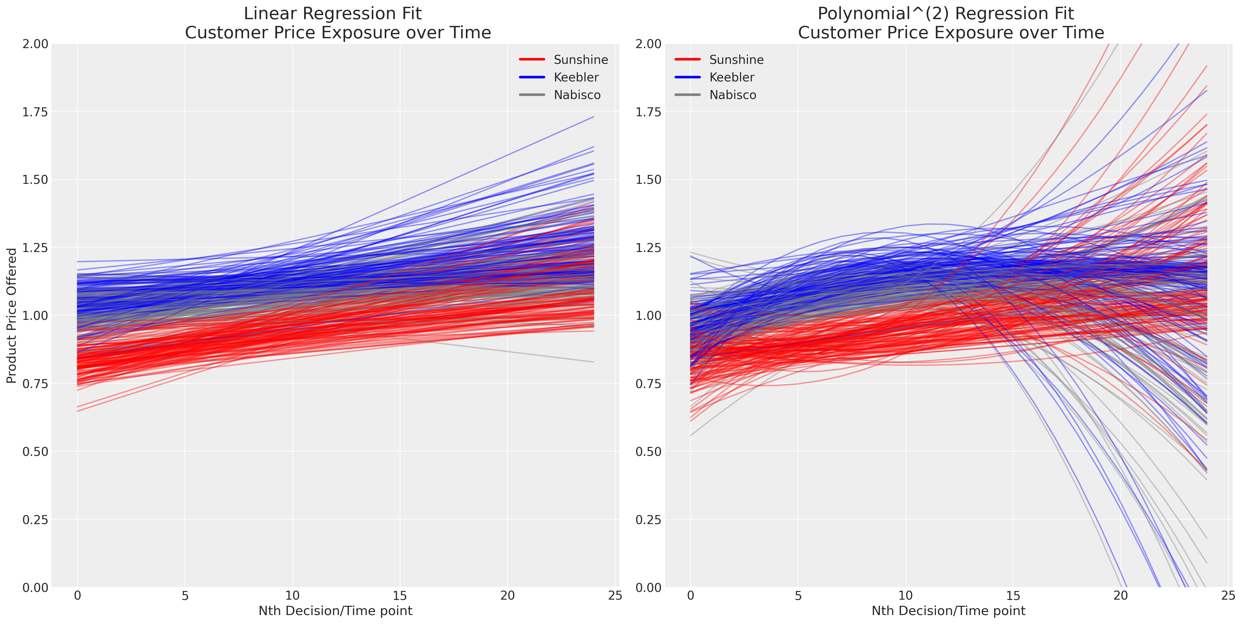
随着时间的推移,重复选择的存在使问题复杂化。我们现在必须处理个人品味以及竞争环境中定价的演变或动态影响等问题。绘制每个人连续接触品牌价格的简单线性和多项式拟合似乎表明 (a) 定价区分了产品供应,并且 (b) 定价随时间演变。
fig, axs = plt.subplots(1, 2, figsize=(20, 10))
axs = axs.flatten()
map_color = {"nabisco": "red", "keebler": "blue", "sunshine": "purple", "private": "orange"}


for i in c_df["personId"].unique():
    temp = c_df[c_df["personId"] == i].copy(deep=True)
    temp["color"] = temp["choice"].map(map_color)
    predict = np.poly1d(np.polyfit(temp["personChoiceId"], temp["price.sunshine"], deg=1))
    axs[0].plot(predict(range(25)), color="red", label="Sunshine", alpha=0.4)
    predict = np.poly1d(np.polyfit(temp["personChoiceId"], temp["price.keebler"], deg=1))
    axs[0].plot(predict(range(25)), color="blue", label="Keebler", alpha=0.4)
    predict = np.poly1d(np.polyfit(temp["personChoiceId"], temp["price.nabisco"], deg=1))
    axs[0].plot(predict(range(25)), color="grey", label="Nabisco", alpha=0.4)

    predict = np.poly1d(np.polyfit(temp["personChoiceId"], temp["price.sunshine"], deg=2))
    axs[1].plot(predict(range(25)), color="red", label="Sunshine", alpha=0.4)
    predict = np.poly1d(np.polyfit(temp["personChoiceId"], temp["price.keebler"], deg=2))
    axs[1].plot(predict(range(25)), color="blue", label="Keebler", alpha=0.4)
    predict = np.poly1d(np.polyfit(temp["personChoiceId"], temp["price.nabisco"], deg=2))
    axs[1].plot(predict(range(25)), color="grey", label="Nabisco", alpha=0.4)

axs[0].set_title("Linear Regression Fit \n Customer Price Exposure over Time", fontsize=20)
axs[1].set_title("Polynomial^(2) Regression Fit \n Customer Price Exposure over Time", fontsize=20)
axs[0].set_xlabel("Nth Decision/Time point")
axs[1].set_xlabel("Nth Decision/Time point")
axs[0].set_ylabel("Product Price Offered")
axs[1].set_ylim(0, 2)
axs[0].set_ylim(0, 2)

colors = ["red", "blue", "grey"]
lines = [Line2D([0], [0], color=c, linewidth=3, linestyle="-") for c in colors]
labels = ["Sunshine", "Keebler", "Nabisco"]
axs[0].legend(lines, labels)
axs[1].legend(lines, labels);
我们现在将建模个人品味如何进入离散选择问题,但忽略时间维度或系统中价格内生性的复杂性。基本离散选择模型有一些调整,旨在解决这些复杂性中的每一个。我们将时间动态留给读者作为建议的练习。
N = c_df.shape[0]
map = {"sunshine": 0, "keebler": 1, "nabisco": 2, "private": 3}
c_df["choice_encoded"] = c_df["choice"].map(map)
observed = c_df["choice_encoded"].values
person_indx, uniques = pd.factorize(c_df["personId"])

coords = {
    "alts_intercepts": ["sunshine", "keebler", "nabisco", "private"],
    "alts_probs": ["sunshine", "keebler", "nabisco", "private"],
    "individuals": uniques,
    "obs": range(N),
}
with pm.Model(coords=coords) as model_4:
    beta_feat = pm.Normal("beta_feat", 0, 1)
    beta_disp = pm.Normal("beta_disp", 0, 1)
    beta_price = pm.Normal("beta_price", 0, 1)
    alphas = pm.Normal("alpha", 0, 1, dims="alts_intercepts")
    ## Hierarchical parameters for individual taste
    beta_individual = pm.Normal("beta_individual", 0, 0.1, dims=("individuals", "alts_intercepts"))

    u0 = (
        (alphas[0] + beta_individual[person_indx, 0])
        + beta_disp * c_df["disp.sunshine"]
        + beta_feat * c_df["feat.sunshine"]
        + beta_price * c_df["price.sunshine"]
    )
    u1 = (
        (alphas[1] + beta_individual[person_indx, 1])
        + beta_disp * c_df["disp.keebler"]
        + beta_feat * c_df["feat.keebler"]
        + beta_price * c_df["price.keebler"]
    )
    u2 = (
        (alphas[2] + beta_individual[person_indx, 2])
        + beta_disp * c_df["disp.nabisco"]
        + beta_feat * c_df["feat.nabisco"]
        + beta_price * c_df["price.nabisco"]
    )
    u3 = (
        (0 + beta_individual[person_indx, 2])
        + beta_disp * c_df["disp.private"]
        + beta_feat * c_df["feat.private"]
        + beta_price * c_df["price.private"]
    )
    s = pm.math.stack([u0, u1, u2, u3]).T

    ## Apply Softmax Transform
    p_ = pm.Deterministic("p", pm.math.softmax(s, axis=1), dims=("obs", "alts_probs"))

    ## Likelihood
    choice_obs = pm.Categorical("y_cat", p=p_, observed=observed, dims="obs")

    idata_m4 = pm.sample_prior_predictive()
    idata_m4.extend(
        pm.sample(nuts_sampler="numpyro", idata_kwargs={"log_likelihood": True}, random_seed=103)
    )
    idata_m4.extend(pm.sample_posterior_predictive(idata_m4))


pm.model_to_graphviz(model_4)
Sampling: [alpha, beta_disp, beta_feat, beta_individual, beta_price, y_cat]
/Users/nathanielforde/mambaforge/envs/pymc_examples_new/lib/python3.9/site-packages/pymc/sampling/mcmc.py:243: UserWarning: Use of external NUTS sampler is still experimental
  warnings.warn("Use of external NUTS sampler is still experimental", UserWarning)
Compiling...
Compilation time =  0:00:01.425976
Sampling...
Sampling time =  0:00:12.028729
Transforming variables...
Transformation time =  0:00:01.427529
Computing Log Likelihood...
Sampling: [y_cat]
Log Likelihood time = 0:00:01.775443

az.summary(idata_m4, var_names=["beta_disp", "beta_feat", "beta_price", "alpha"]).head(6)
| 平均值 | 标准差 | hdi_3% | hdi_97% | mcse_mean | mcse_sd | ess_bulk | ess_tail | r_hat | |
|---|---|---|---|---|---|---|---|---|---|
| beta_disp | 0.104 | 0.063 | -0.016 | 0.216 | 0.001 | 0.001 | 5853.0 | 3169.0 | 1.00 |
| beta_feat | 0.505 | 0.095 | 0.325 | 0.678 | 0.001 | 0.001 | 4476.0 | 2663.0 | 1.00 |
| beta_price | -2.977 | 0.209 | -3.395 | -2.607 | 0.005 | 0.004 | 1765.0 | 2557.0 | 1.00 |
| alpha[sunshine] | -0.708 | 0.093 | -0.883 | -0.531 | 0.002 | 0.001 | 2493.0 | 2960.0 | 1.00 |
| alpha[keebler] | -0.231 | 0.120 | -0.449 | 0.000 | 0.003 | 0.002 | 1974.0 | 2635.0 | 1.00 |
| alpha[nabisco] | 1.723 | 0.101 | 1.538 | 1.920 | 0.002 | 0.002 | 1752.0 | 2653.0 | 1.01 |
我们学到了什么?我们对价格系数施加了负斜率,但赋予了它广泛的先验。我们可以看到,数据足以大大缩小系数的可能范围。
az.plot_dist_comparison(idata_m4, var_names=["beta_price"]);
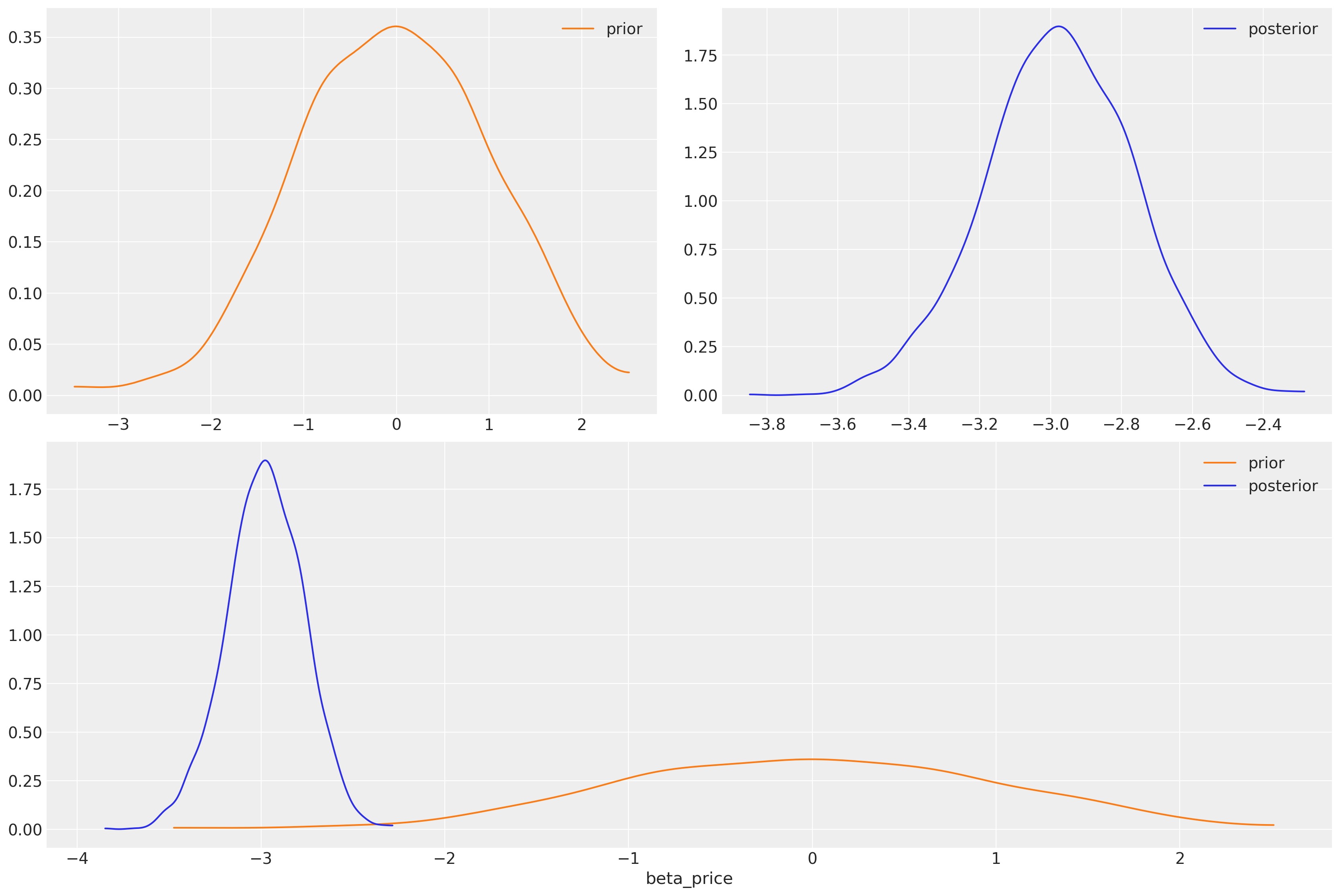
我们已经恢复了与理性选择基本理论一致的价格效应的强烈负估计。价格效应应该对效用产生负面影响。先验的灵活性是在此设置中结合有关选择过程的理论知识的关键。先验对于构建更好的决策过程图景非常重要,而我们忽略它们在这种设置中的价值是愚蠢的。
fig, axs = plt.subplots(1, 2, figsize=(20, 10))
ax = axs[0]
counts = c_df.groupby("choice")["choiceId"].count()
labels = c_df.groupby("choice")["choiceId"].count().index
predicted_shares = idata_m4["posterior"]["p"].mean(dim=["chain", "draw", "obs"])
ci_lb = idata_m4["posterior"]["p"].quantile(0.025, dim=["chain", "draw", "obs"])
ci_ub = idata_m4["posterior"]["p"].quantile(0.975, dim=["chain", "draw", "obs"])
ax.scatter(ci_lb, labels, color="k", s=2)
ax.scatter(ci_ub, labels, color="k", s=2)
ax.scatter(
    counts / counts.sum(),
    labels,
    label="Observed Shares",
    color="red",
    s=100,
)
ax.scatter(
    predicted_shares,
    predicted_shares["alts_probs"].values,
    label="Predicted Mean",
    color="green",
    s=200,
    alpha=0.5,
)
ax.hlines(
    predicted_shares["alts_probs"].values,
    ci_lb,
    ci_ub,
    label="Predicted 95% Interval",
    color="black",
)
ax.legend()
ax.set_title("Observed V Predicted Shares")
az.plot_ppc(idata_m4, ax=axs[1])
axs[1].set_title("Posterior Predictive Checks")
ax.set_xlabel("Shares")
ax.set_ylabel("Crackers");
/Users/nathanielforde/mambaforge/envs/pymc_examples_new/lib/python3.9/site-packages/arviz/plots/ppcplot.py:267: FutureWarning: The return type of `Dataset.dims` will be changed to return a set of dimension names in future, in order to be more consistent with `DataArray.dims`. To access a mapping from dimension names to lengths, please use `Dataset.sizes`.
  flatten_pp = list(predictive_dataset.dims.keys())
/Users/nathanielforde/mambaforge/envs/pymc_examples_new/lib/python3.9/site-packages/arviz/plots/ppcplot.py:271: FutureWarning: The return type of `Dataset.dims` will be changed to return a set of dimension names in future, in order to be more consistent with `DataArray.dims`. To access a mapping from dimension names to lengths, please use `Dataset.sizes`.
  flatten = list(observed_data.dims.keys())
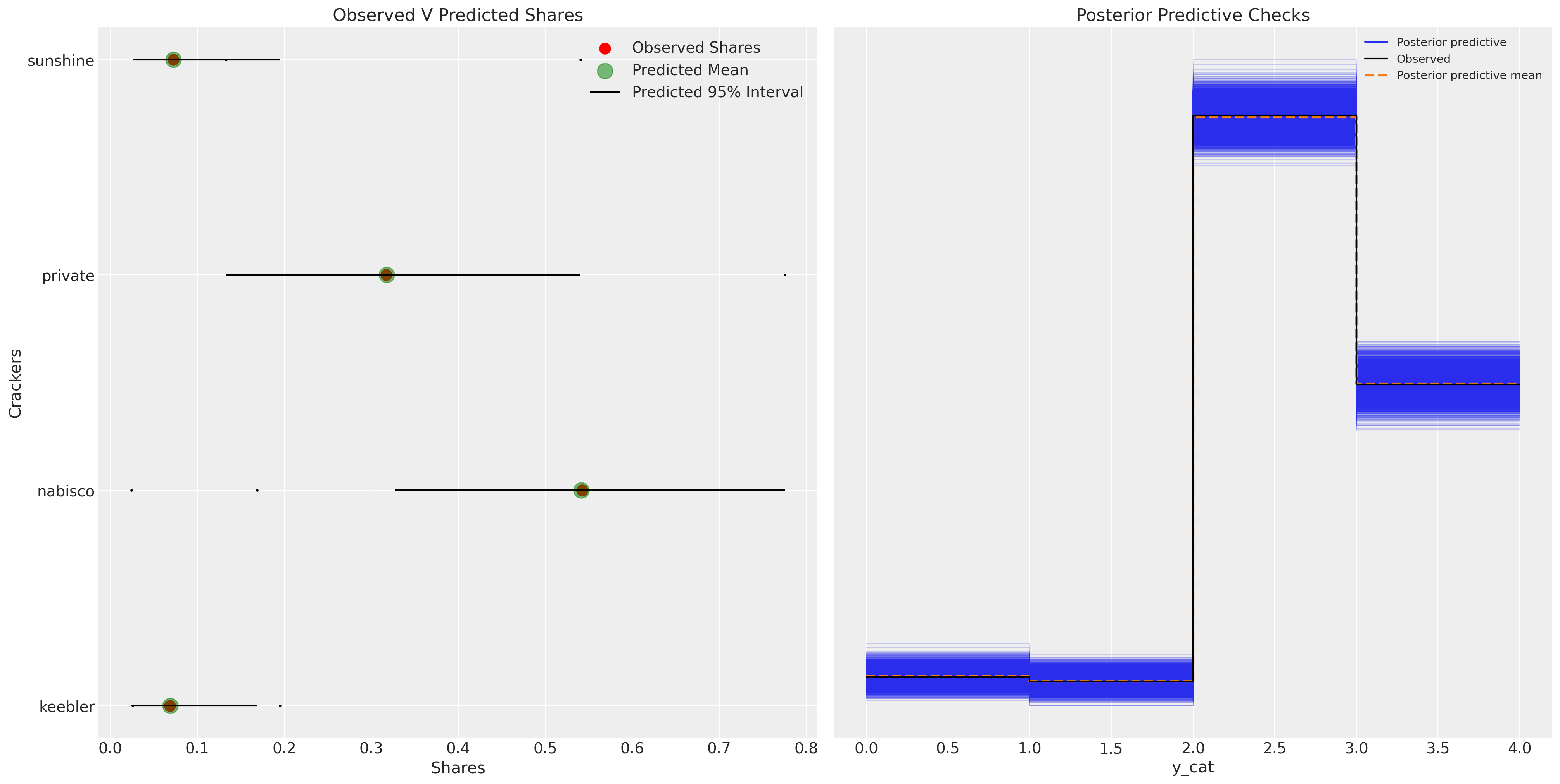
我们现在还可以恢复模型估计的个体之间对于特定饼干选择的差异。更准确地说,我们将绘制个体特定贡献如何影响饼干选择之间的偏好。
idata_m4
-
<xarray.Dataset> Dimensions: (chain: 4, draw: 1000, alts_intercepts: 4, individuals: 136, obs: 3156, alts_probs: 4) Coordinates: * chain (chain) int64 0 1 2 3 * draw (draw) int64 0 1 2 3 4 5 6 ... 993 994 995 996 997 998 999 * alts_intercepts (alts_intercepts) <U8 'sunshine' 'keebler' ... 'private' * individuals (individuals) int64 1 2 3 4 5 6 ... 131 132 133 134 135 136 * obs (obs) int64 0 1 2 3 4 5 6 ... 3150 3151 3152 3153 3154 3155 * alts_probs (alts_probs) <U8 'sunshine' 'keebler' 'nabisco' 'private' Data variables: beta_feat (chain, draw) float64 0.5783 0.4997 ... 0.4685 0.3407 beta_disp (chain, draw) float64 0.05753 0.1059 ... 0.02148 0.02866 beta_price (chain, draw) float64 -3.17 -3.142 -2.818 ... -2.835 -3.0 alpha (chain, draw, alts_intercepts) float64 -0.6961 ... 1.907 beta_individual (chain, draw, individuals, alts_intercepts) float64 -0.0... p (chain, draw, obs, alts_probs) float64 0.05034 ... 0.4659 Attributes: created_at: 2025-03-22T20:12:22.857603 arviz_version: 0.17.0 -
<xarray.Dataset> Dimensions: (chain: 4, draw: 1000, obs: 3156) Coordinates: * chain (chain) int64 0 1 2 3 * draw (draw) int64 0 1 2 3 4 5 6 7 8 ... 992 993 994 995 996 997 998 999 * obs (obs) int64 0 1 2 3 4 5 6 7 ... 3149 3150 3151 3152 3153 3154 3155 Data variables: y_cat (chain, draw, obs) int64 2 1 2 2 0 1 2 2 3 0 ... 2 1 3 3 3 3 3 3 2 Attributes: created_at: 2025-03-22T20:12:46.931302 arviz_version: 0.17.0 inference_library: pymc inference_library_version: 5.3.0 -
<xarray.Dataset> Dimensions: (chain: 4, draw: 1000, y_cat_dim_0: 1, y_cat_dim_1: 3156) Coordinates: * chain (chain) int64 0 1 2 3 * draw (draw) int64 0 1 2 3 4 5 6 7 ... 993 994 995 996 997 998 999 * y_cat_dim_0 (y_cat_dim_0) int64 0 * y_cat_dim_1 (y_cat_dim_1) int64 0 1 2 3 4 5 ... 3151 3152 3153 3154 3155 Data variables: y_cat (chain, draw, y_cat_dim_0, y_cat_dim_1) float64 -0.4611 ... ... Attributes: created_at: 2025-03-22T20:12:22.862153 arviz_version: 0.17.0 -
<xarray.Dataset> Dimensions: (chain: 4, draw: 1000) Coordinates: * chain (chain) int64 0 1 2 3 * draw (draw) int64 0 1 2 3 4 5 6 ... 993 994 995 996 997 998 999 Data variables: acceptance_rate (chain, draw) float64 0.591 0.8318 0.8023 ... 0.9768 0.9868 step_size (chain, draw) float64 0.2807 0.2807 ... 0.2612 0.2612 diverging (chain, draw) bool False False False ... False False False energy (chain, draw) float64 3.003e+03 2.971e+03 ... 3.043e+03 n_steps (chain, draw) int64 15 15 15 15 15 15 ... 15 15 15 15 15 15 tree_depth (chain, draw) int64 4 4 4 4 4 4 4 4 4 ... 4 4 4 4 4 4 4 4 4 lp (chain, draw) float64 2.698e+03 2.706e+03 ... 2.741e+03 Attributes: created_at: 2025-03-22T20:12:22.860838 arviz_version: 0.17.0 -
<xarray.Dataset> Dimensions: (chain: 1, draw: 500, alts_intercepts: 4, obs: 3156, alts_probs: 4, individuals: 136) Coordinates: * chain (chain) int64 0 * draw (draw) int64 0 1 2 3 4 5 6 ... 493 494 495 496 497 498 499 * alts_intercepts (alts_intercepts) <U8 'sunshine' 'keebler' ... 'private' * obs (obs) int64 0 1 2 3 4 5 6 ... 3150 3151 3152 3153 3154 3155 * alts_probs (alts_probs) <U8 'sunshine' 'keebler' 'nabisco' 'private' * individuals (individuals) int64 1 2 3 4 5 6 ... 131 132 133 134 135 136 Data variables: alpha (chain, draw, alts_intercepts) float64 1.072 ... -0.2998 beta_price (chain, draw) float64 -1.56 -1.028 0.3816 ... -0.5425 -1.41 p (chain, draw, obs, alts_probs) float64 0.4438 ... 0.5711 beta_individual (chain, draw, individuals, alts_intercepts) float64 -0.0... beta_disp (chain, draw) float64 -0.1106 -0.604 ... 0.1959 -0.846 beta_feat (chain, draw) float64 1.538 0.0226 ... 0.3186 -0.3146 Attributes: created_at: 2025-03-22T20:12:05.460153 arviz_version: 0.17.0 inference_library: pymc inference_library_version: 5.3.0 -
<xarray.Dataset> Dimensions: (chain: 1, draw: 500, obs: 3156) Coordinates: * chain (chain) int64 0 * draw (draw) int64 0 1 2 3 4 5 6 7 8 ... 492 493 494 495 496 497 498 499 * obs (obs) int64 0 1 2 3 4 5 6 7 ... 3149 3150 3151 3152 3153 3154 3155 Data variables: y_cat (chain, draw, obs) int64 0 0 2 3 1 3 0 1 3 0 ... 2 3 3 1 3 1 3 3 3 Attributes: created_at: 2025-03-22T20:12:05.463770 arviz_version: 0.17.0 inference_library: pymc inference_library_version: 5.3.0 -
<xarray.Dataset>
Dimensions:  (obs: 3156)
Coordinates:
  * obs      (obs) int64 0 1 2 3 4 5 6 7 ... 3149 3150 3151 3152 3153 3154 3155
Data variables:
    y_cat    (obs) int64 2 0 2 2 2 0 2 2 2 2 2 2 2 ... 3 3 0 3 3 3 3 3 3 3 3 3 3
Attributes:
    created_at:                 2025-03-22T20:12:05.464353
    arviz_version:              0.17.0
    inference_library:          pymc
    inference_library_version:  5.3.0
beta_individual = idata_m4["posterior"]["beta_individual"]
predicted = beta_individual.mean(("chain", "draw"))
predicted = predicted.sortby(predicted.sel(alts_intercepts="nabisco"))
ci_lb = beta_individual.quantile(0.025, ("chain", "draw")).sortby(
    predicted.sel(alts_intercepts="nabisco")
)
ci_ub = beta_individual.quantile(0.975, ("chain", "draw")).sortby(
    predicted.sel(alts_intercepts="nabisco")
)
fig = plt.figure(figsize=(10, 9))
gs = fig.add_gridspec(
    2,
    3,
    width_ratios=(4, 4, 4),
    height_ratios=(1, 7),
    left=0.1,
    right=0.9,
    bottom=0.1,
    top=0.9,
    wspace=0.05,
    hspace=0.05,
)
# Create the Axes.
ax = fig.add_subplot(gs[1, 0])
ax.set_yticklabels([])
ax_histx = fig.add_subplot(gs[0, 0], sharex=ax)
ax_histx.set_title("Expected Modifications \n to Nabisco Baseline", fontsize=10)
ax_histx.hist(predicted.sel(alts_intercepts="nabisco"), bins=30, ec="black", color="red")
ax_histx.set_yticklabels([])
ax_histx.tick_params(labelsize=8)
ax.set_ylabel("Individuals", fontsize=10)
ax.tick_params(labelsize=8)
ax.hlines(
    range(len(predicted)),
    ci_lb.sel(alts_intercepts="nabisco"),
    ci_ub.sel(alts_intercepts="nabisco"),
    color="black",
    alpha=0.3,
)
ax.scatter(predicted.sel(alts_intercepts="nabisco"), range(len(predicted)), color="red", ec="white")
ax.fill_betweenx(range(139), -0.03, 0.03, alpha=0.2, color="red")

ax1 = fig.add_subplot(gs[1, 1])
ax1.set_yticklabels([])
ax_histx = fig.add_subplot(gs[0, 1], sharex=ax1)
ax_histx.set_title("Expected Modifications \n to Keebler Baseline", fontsize=10)
ax_histx.set_yticklabels([])
ax_histx.tick_params(labelsize=8)
ax_histx.hist(predicted.sel(alts_intercepts="keebler"), bins=30, ec="black", color="red")
ax1.hlines(
    range(len(predicted)),
    ci_lb.sel(alts_intercepts="keebler"),
    ci_ub.sel(alts_intercepts="keebler"),
    color="black",
    alpha=0.3,
)
ax1.scatter(
    predicted.sel(alts_intercepts="keebler"), range(len(predicted)), color="red", ec="white"
)
ax1.set_xlabel("Individual Modifications to the Product Intercept", fontsize=10)
ax1.fill_betweenx(range(139), -0.03, 0.03, alpha=0.2, color="red", label="Negligible \n Region")
ax1.tick_params(labelsize=8)
ax1.legend(fontsize=10)

ax2 = fig.add_subplot(gs[1, 2])
ax2.set_yticklabels([])
ax_histx = fig.add_subplot(gs[0, 2], sharex=ax2)
ax_histx.set_title("Expected Modifications \n to Sunshine Baseline", fontsize=10)
ax_histx.set_yticklabels([])
ax_histx.hist(predicted.sel(alts_intercepts="sunshine"), bins=30, ec="black", color="red")
ax2.hlines(
    range(len(predicted)),
    ci_lb.sel(alts_intercepts="sunshine"),
    ci_ub.sel(alts_intercepts="sunshine"),
    color="black",
    alpha=0.3,
)
ax2.fill_betweenx(range(139), -0.03, 0.03, alpha=0.2, color="red")
ax2.scatter(
    predicted.sel(alts_intercepts="sunshine"), range(len(predicted)), color="red", ec="white"
)
ax2.tick_params(labelsize=8)
ax_histx.tick_params(labelsize=8)
plt.suptitle("Individual Differences by Product", fontsize=20);
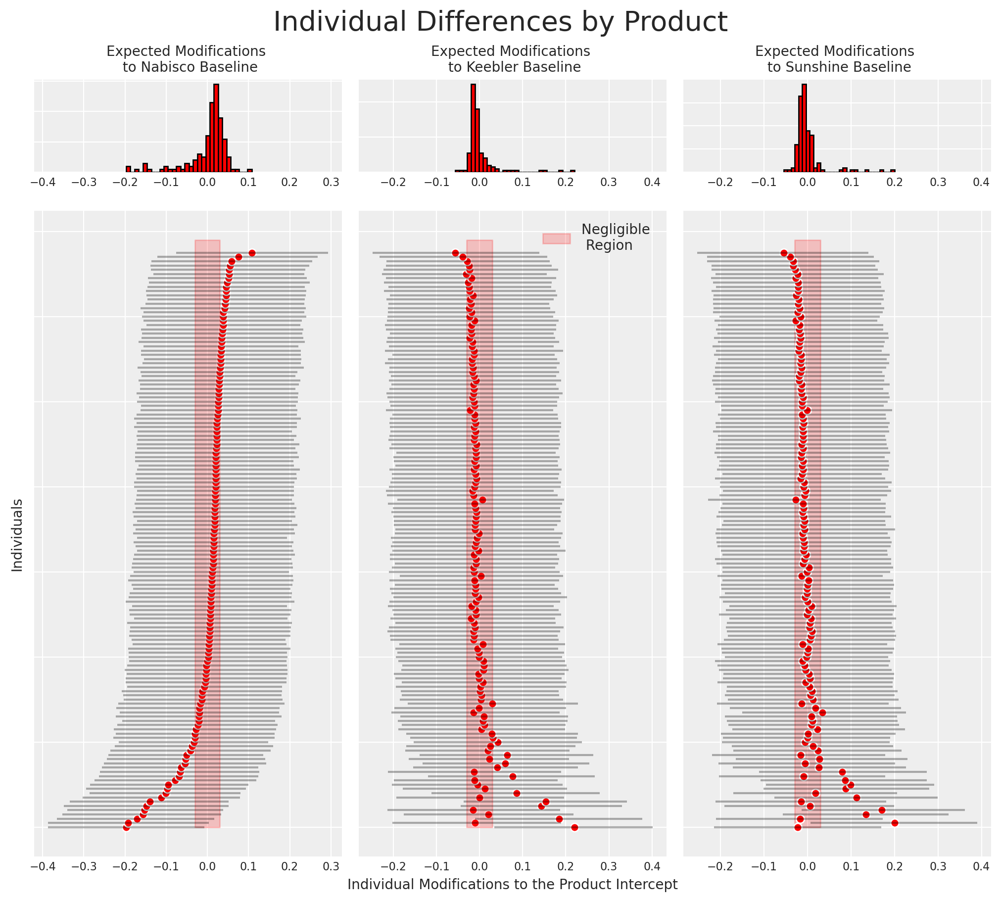
这种类型的图通常用于识别忠诚客户。同样,如果我们希望他们转向我们的产品,它也可以用于识别应该更好地激励的客户群体。
结论#
我们在此可以看到建模离散选项的个人选择的灵活性和丰富的参数化可能性。 这些技术在从微观经济学到市场营销和产品开发的广泛领域都非常有用。 效用、概率及其相互作用的概念是 萨维奇表示定理 和贝叶斯统计推断方法的合理性论证的核心。 因此,离散建模自然适合贝叶斯方法,而贝叶斯统计也自然适合离散选择建模。 传统的估计技术通常很脆弱,并且非常依赖 MLE 过程的起始值。 贝叶斯设置用一个框架取代了这种脆弱性,该框架允许我们纳入我们对驱动人类效用计算的因素的信念。 在这个示例 notebook 中,我们只是浅尝辄止,但鼓励您进一步探索这项技术。
参考文献#
水印#
%load_ext watermark
%watermark -n -u -v -iv -w -p pytensor
Last updated: Sat Mar 22 2025

Python implementation: CPython
Python version       : 3.9.16
IPython version      : 8.12.0

pytensor: 2.11.1

numpy     : 1.24.4
pytensor  : 2.11.1
pymc      : 5.3.0
matplotlib: 3.8.2
arviz     : 0.17.0
pandas    : 1.5.3

Watermark: 2.3.1
许可声明#
此示例库中的所有 notebook 均根据 MIT 许可证 提供,该许可证允许修改和再分发以用于任何用途,前提是版权和许可声明得到保留。
引用 PyMC 示例#
要引用此 notebook,请使用 Zenodo 为 pymc-examples 存储库提供的 DOI。
重要提示
许多 notebook 改编自其他来源:博客、书籍... 在这种情况下,您也应该引用原始来源。
另请记住引用您的代码使用的相关库。
这是一个 bibtex 格式的引用模板
@incollection{citekey,
  author    = "<notebook authors, see above>",
  title     = "<notebook title>",
  editor    = "PyMC Team",
  booktitle = "PyMC examples",
  doi       = "10.5281/zenodo.5654871"
}
渲染后可能看起来像这样