GLM：模型选择#

import arviz as az
import bambi as bmb
import matplotlib.pyplot as plt
import numpy as np
import pandas as pd
import pymc as pm
import seaborn as sns
import xarray as xr

from ipywidgets import fixed, interactive

print(f"Running on PyMC v{pm.__version__}")

Running on PyMC v5.19.1

RANDOM_SEED = 8927
rng = np.random.default_rng(RANDOM_SEED)

%config InlineBackend.figure_format = 'retina'
az.style.use("arviz-darkgrid")
plt.rcParams["figure.constrained_layout.use"] = False

简介#

一个相当简洁的可复现示例，展示了如何在 PyMC 中使用 WAIC 和 LOO 进行模型选择。

本示例创建了在线性和二次模型下的两个玩具数据集，然后通过使用广泛应用的信息准则 (WAIC) 和留一法 (LOO) 交叉验证（使用 Pareto 平滑重要性抽样 (PSIS)），测试了一系列多项式线性模型对这些数据集的拟合程度。

该示例的灵感来自 Jake Vanderplas 关于模型选择的博客文章，尽管交叉验证和贝叶斯因子比较尚未实现。数据集很小，在本 Notebook 中生成。它们仅包含测量值 (y) 中的误差。

局部函数#

我们开始编写一些函数来帮助完成 Notebook 的其余部分。只有一些函数是理解 Notebook 的关键，其余的是为了在需要时使绘图更简洁的便利函数，并隐藏在可切换的部分中；它仍然可用，但您需要单击才能看到它。

def generate_data(n=20, p=0, a=1, b=1, c=0, latent_sigma_y=20, seed=5):
    """
    Create a toy dataset based on a very simple model that we might
    imagine is a noisy physical process:
        1. random x values within a range
        2. latent error aka inherent noise in y
        3. optionally create labelled outliers with larger noise

    Model form: y ~ a + bx + cx^2 + e

    NOTE: latent_sigma_y is used to create a normally distributed,
    'latent error' aka 'inherent noise' in the 'physical' generating
    process, rather than experimental measurement error.
    Please don't use the returned `latent_error` values in inferential
    models, it's returned in the dataframe for interest only.
    """
    rng = np.random.default_rng(seed)
    df = pd.DataFrame({"x": rng.choice(np.arange(100), n, replace=False)})

    # create linear or quadratic model
    df["y"] = a + b * (df["x"]) + c * (df["x"]) ** 2

    # create latent noise and marked outliers
    df["latent_error"] = rng.normal(0, latent_sigma_y, n)
    df["outlier_error"] = rng.normal(0, latent_sigma_y * 10, n)
    df["outlier"] = rng.binomial(1, p, n)

    # add noise, with extreme noise for marked outliers
    df["y"] += (1 - df["outlier"]) * df["latent_error"]
    df["y"] += df["outlier"] * df["outlier_error"]

    # round
    for col in ["y", "latent_error", "outlier_error", "x"]:
        df[col] = np.round(df[col], 3)

    # add label
    df["source"] = "linear" if c == 0 else "quadratic"

    # create simple linspace for plotting true model
    plotx = np.linspace(
        df["x"].min() - np.ptp(df["x"].values) * 0.1,
        df["x"].max() + np.ptp(df["x"].values) * 0.1,
        100,
    )

    ploty = a + b * plotx + c * plotx**2
    dfp = pd.DataFrame({"x": plotx, "y": ploty})

    return df, dfp

显示代码单元格内容隐藏代码单元格内容

def interact_dataset(n=20, p=0, a=-30, b=5, c=0, latent_sigma_y=20):
    """
    Convenience function:
    Interactively generate dataset and plot
    """

    df, dfp = generate_data(n, p, a, b, c, latent_sigma_y)

    g = sns.FacetGrid(
        df,
        height=8,
        hue="outlier",
        hue_order=[True, False],
        palette=sns.color_palette("bone"),
        legend_out=False,
    )

    g.map(
        plt.errorbar,
        "x",
        "y",
        "latent_error",
        marker="o",
        ms=10,
        mec="w",
        mew=2,
        ls="",
        elinewidth=0.7,
    ).add_legend()

    plt.plot(dfp["x"], dfp["y"], "--", alpha=0.8)

    plt.subplots_adjust(top=0.92)
    g.fig.suptitle("Sketch of Data Generation ({})".format(df["source"][0]), fontsize=16)


def plot_datasets(df_lin, df_quad, dfp_lin, dfp_quad):
    """
    Convenience function:
    Plot the two generated datasets in facets with generative model
    """

    df = pd.concat((df_lin, df_quad), axis=0)

    g = sns.FacetGrid(col="source", hue="source", data=df, height=6, sharey=False, legend_out=False)

    g.map(plt.scatter, "x", "y", alpha=0.7, s=100, lw=2, edgecolor="w")

    g.axes[0][0].plot(dfp_lin["x"], dfp_lin["y"], "--", alpha=0.6, color="C0")
    g.axes[0][1].plot(dfp_quad["x"], dfp_quad["y"], "--", alpha=0.6, color="C0")


def plot_annotated_trace(traces):
    """
    Convenience function:
    Plot traces with overlaid means and values
    """

    summary = az.summary(traces, stat_funcs={"mean": np.mean}, extend=False)
    ax = az.plot_trace(
        traces,
        lines=tuple([(k, {}, v["mean"]) for k, v in summary.iterrows()]),
    )

    for i, mn in enumerate(summary["mean"].values):
        ax[i, 0].annotate(
            f"{mn:.2f}",
            xy=(mn, 0),
            xycoords="data",
            xytext=(5, 10),
            textcoords="offset points",
            rotation=90,
            va="bottom",
            fontsize="large",
            color="C0",
        )


def plot_posterior_cr(models, idatas, rawdata, xlims, datamodelnm="linear", modelnm="k1"):
    """
    Convenience function:
    Plot posterior predictions with credible regions shown as filled areas.
    """

    # Get traces and calc posterior prediction for npoints in x
    npoints = 100
    mdl = models[modelnm]
    trc = idatas[modelnm].posterior.copy()

    # Extract variables and stack them in correct order
    vars_to_concat = []
    for var in ["Intercept", "x"] + [f"np.power(x, {i})" for i in range(2, int(modelnm[-1:]) + 1)]:
        if var in trc:
            vars_to_concat.append(trc[var])
    da = xr.concat(vars_to_concat, dim="order")

    ordr = len(vars_to_concat)
    x = xr.DataArray(np.linspace(xlims[0], xlims[1], npoints), dims=["x_plot"])
    pwrs = xr.DataArray(np.arange(ordr), dims=["order"])
    X = x**pwrs
    cr = xr.dot(X, da, dims="order")

    # Calculate credible regions and plot over the datapoints
    qs = cr.quantile([0.025, 0.25, 0.5, 0.75, 0.975], dim=("chain", "draw"))

    f, ax1d = plt.subplots(1, 1, figsize=(7, 7))
    f.suptitle(
        f"Posterior Predictive Fit -- Data: {datamodelnm} -- Model: {modelnm}",
        fontsize=16,
    )

    ax1d.fill_between(
        x, qs.sel(quantile=0.025), qs.sel(quantile=0.975), alpha=0.5, color="C0", label="CR 95%"
    )
    ax1d.fill_between(
        x, qs.sel(quantile=0.25), qs.sel(quantile=0.75), alpha=0.5, color="C3", label="CR 50%"
    )
    ax1d.plot(x, qs.sel(quantile=0.5), alpha=0.6, color="C4", label="Median")
    ax1d.scatter(rawdata["x"], rawdata["y"], alpha=0.7, s=100, lw=2, edgecolor="w")

    ax1d.legend()
    ax1d.set_xlim(xlims)

生成玩具数据集#

交互式草拟数据#

在 Notebook 的其余部分，我们将使用分别由线性和二次模型创建的两个玩具数据集，以便我们更好地评估模型选择的拟合度。

现在，让我们使用交互式会话来试用本 Notebook 中的数据生成函数，并了解我们可以生成的数据的可能性。

\[y_{i} = a + bx_{i} + cx_{i}^{2} + \epsilon_{i}\]

其中
\(i \in n\) 数据点

\[\epsilon \sim \mathcal{N}(0,latent\_sigma\_y)\]

关于异常值的说明

我们可以使用值 p 来设置伯努利分布下“异常值”的（近似）比例。
这些异常值的 latent_sigma_y 大 10 倍
这些异常值在返回的数据集中被标记，可能对其他建模有用，请参阅另一个示例 Notebook：GLM：使用自定义似然函数进行异常值分类的稳健回归

interactive(
    interact_dataset,
    n=[5, 50, 5],
    p=[0, 0.5, 0.05],
    a=[-50, 50],
    b=[-10, 10],
    c=[-3, 3],
    latent_sigma_y=[0, 1000, 50],
)

观察

我已在误差条中显示了 latent_error，但这仅供参考，因为它显示了我们想象创建数据的任何“物理过程”中的固有噪声。
没有测量误差。
作为异常值创建的数据点以红色显示，同样仅供参考。

创建用于建模的数据集#

我们可以使用上面的交互式绘图来感受参数的效果。现在我们将创建 2 个固定的数据集，用于 Notebook 的其余部分。

首先，我们将创建一个具有小噪声的线性模型。保持简单。
其次，一个具有小噪声的二次模型

n = 30
df_lin, dfp_lin = generate_data(n=n, p=0, a=-30, b=5, c=0, latent_sigma_y=40, seed=RANDOM_SEED)
df_quad, dfp_quad = generate_data(n=n, p=0, a=-200, b=2, c=3, latent_sigma_y=500, seed=RANDOM_SEED)

针对模型线的散点图

plot_datasets(df_lin, df_quad, dfp_lin, dfp_quad)

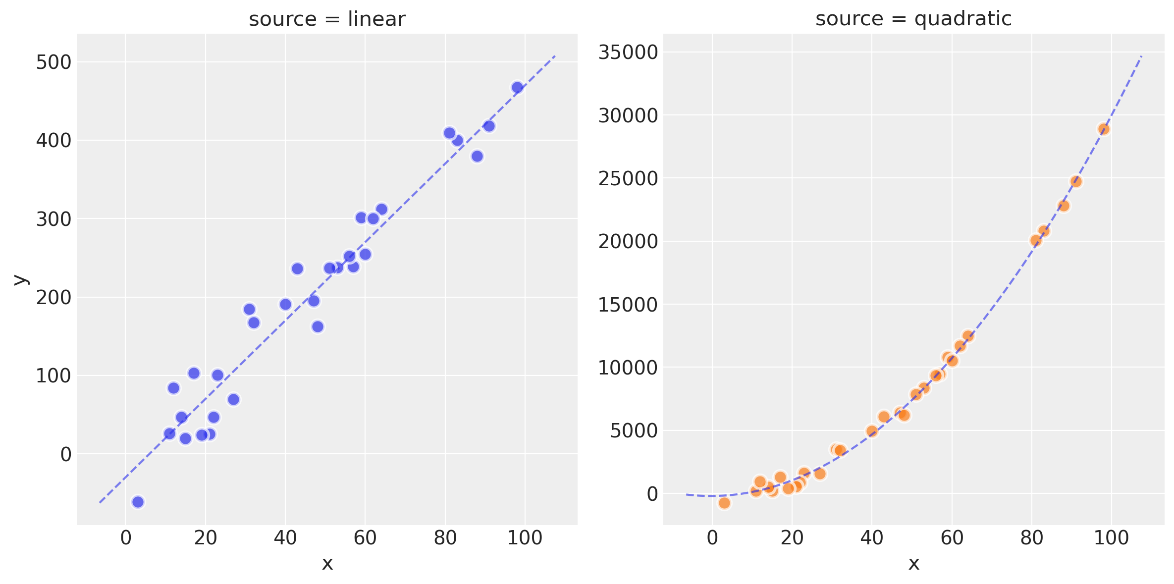
../_images/2abb4b985087a1a8d5f8dfa5b485b34f0134adcceb8cccb3fc9dc0f31ada9047.png

观察

我们现在有两个数据集 df_lin 和 df_quad，分别由线性模型和二次模型创建。
您可以在上面的散点图中看到原始数据、理想的模型拟合以及潜在噪声的影响
在本 Notebook 的后续绘图中，线性生成的数据将以蓝色显示，二次数据将以绿色显示。

标准化#

dfs_lin = df_lin.copy()
dfs_lin["x"] = (df_lin["x"] - df_lin["x"].mean()) / df_lin["x"].std()

dfs_quad = df_quad.copy()
dfs_quad["x"] = (df_quad["x"] - df_quad["x"].mean()) / df_quad["x"].std()

创建范围以供稍后使用 ylim xim

dfs_lin_xlims = (
    dfs_lin["x"].min() - np.ptp(dfs_lin["x"].values) / 10,
    dfs_lin["x"].max() + np.ptp(dfs_lin["x"].values) / 10,
)

dfs_lin_ylims = (
    dfs_lin["y"].min() - np.ptp(dfs_lin["y"].values) / 10,
    dfs_lin["y"].max() + np.ptp(dfs_lin["y"].values) / 10,
)

dfs_quad_ylims = (
    dfs_quad["y"].min() - np.ptp(dfs_quad["y"].values) / 10,
    dfs_quad["y"].max() + np.ptp(dfs_quad["y"].values) / 10,
)

演示简单线性模型#

这个线性模型非常简单和传统，是一个带有 L2 约束的 OLS（岭回归）

\[y = a + bx + \epsilon\]

使用显式 PyMC 方法定义模型#

with pm.Model() as mdl_ols:
    ## define Normal priors to give Ridge regression
    b0 = pm.Normal("Intercept", mu=0, sigma=100)
    b1 = pm.Normal("x", mu=0, sigma=100)

    ## define Linear model
    yest = b0 + b1 * df_lin["x"]

    ## define Normal likelihood with HalfCauchy noise (fat tails, equiv to HalfT 1DoF)
    y_sigma = pm.HalfCauchy("y_sigma", beta=10)
    likelihood = pm.Normal("likelihood", mu=yest, sigma=y_sigma, observed=df_lin["y"])

    idata_ols = pm.sample(2000, return_inferencedata=True)

Initializing NUTS using jitter+adapt_diag...
Multiprocess sampling (4 chains in 4 jobs)
NUTS: [Intercept, x, y_sigma]

Sampling 4 chains for 1_000 tune and 2_000 draw iterations (4_000 + 8_000 draws total) took 1 seconds.

plt.rcParams["figure.constrained_layout.use"] = True
plot_annotated_trace(idata_ols)

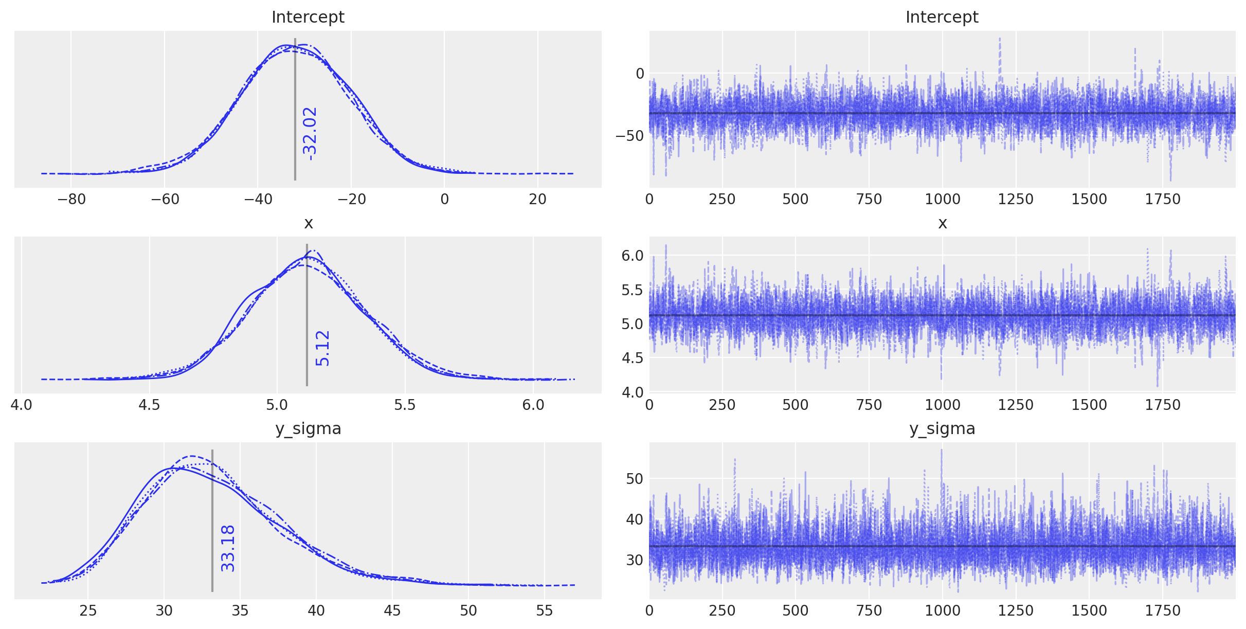
../_images/cf28323a461c7b1b709ed1c21443bfc8f3d43b28681c6cdbc650dc059b96ca11.png

观察

这个简单的 OLS 设法对模型参数做出了相当好的猜测——毕竟数据生成得相当简单——但它似乎确实被固有噪声稍微愚弄了。

使用 Bambi 定义模型#

Bambi 可用于使用 formulae 样式公式语法定义模型。这似乎非常有用，尤其是在用更少的代码行定义简单回归模型时。

这是与上面相同的 OLS 模型，使用 bambi 定义。

# Define priors for intercept and regression coefficients.
priors = {
    "Intercept": bmb.Prior("Normal", mu=0, sigma=100),
    "x": bmb.Prior("Normal", mu=0, sigma=100),
}

model = bmb.Model("y ~ 1 + x", df_lin, priors=priors, family="gaussian")

idata_ols_glm = model.fit(draws=2000, tune=2000)

Initializing NUTS using jitter+adapt_diag...
Multiprocess sampling (4 chains in 4 jobs)
NUTS: [sigma, Intercept, x]

Sampling 4 chains for 2_000 tune and 2_000 draw iterations (8_000 + 8_000 draws total) took 1 seconds.

plot_annotated_trace(idata_ols_glm)

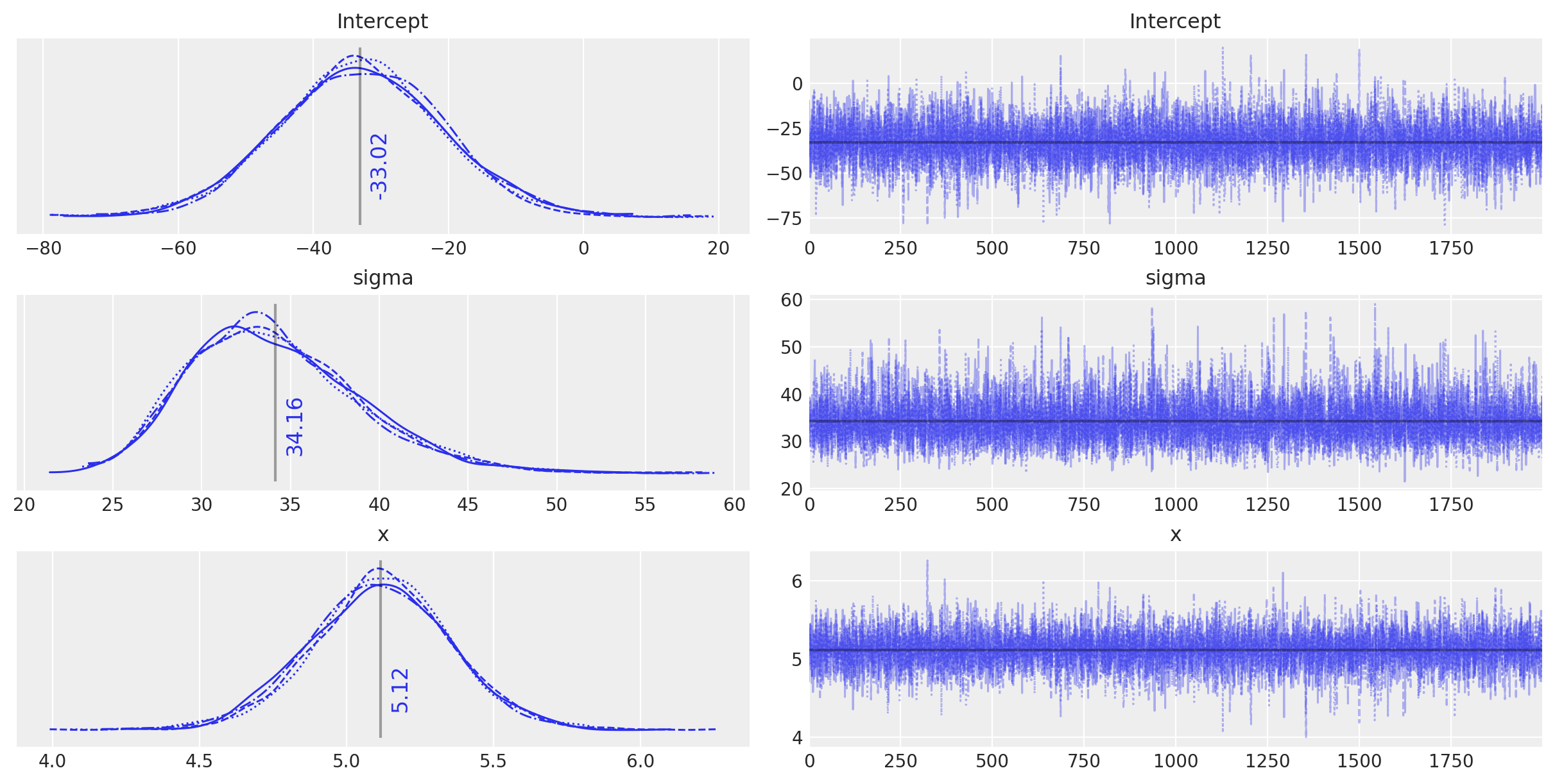
../_images/7bf6b64a0bb9dd51bfcbeebcad850636151f620dd27a2d71f198a17162c6ff41.png

观察

这个 bambi 定义的模型似乎以非常相似的方式运行，并且找到了与传统定义的模型相同的参数值——任何差异都是由于抽样的随机性造成的。
我们可以非常愉快地在下面的进一步模型中使用 bambi 语法，因为它允许我们非常轻松地创建一个小型模型工厂。

创建更高阶的线性模型#

回到本 Notebook 的真正目的，演示模型选择。

首先，让我们在每个玩具数据集上创建并运行一组多项式模型。默认情况下，这是针对 1 到 5 阶的模型。

创建并运行多项式模型#

我们正在创建 5 个多项式模型，并使用下面的函数 create_poly_modelspec 和 run_models 将每个模型拟合到选定的数据集。

def create_poly_modelspec(k=1):
    """
    Convenience function:
    Create a polynomial modelspec string for bambi
    """
    return ("y ~ 1 + x " + " ".join([f"+ np.power(x,{j})" for j in range(2, k + 1)])).strip()


def run_models(df, upper_order=5):
    """
    Convenience function:
    Fit a range of pymc models of increasing polynomial complexity.
    Suggest limit to max order 5 since calculation time is exponential.
    """

    models, results = dict(), dict()

    for k in range(1, upper_order + 1):
        nm = f"k{k}"
        fml = create_poly_modelspec(k)

        print(f"\nRunning: {nm}")

        models[nm] = bmb.Model(
            fml, df, priors={"intercept": bmb.Prior("Normal", mu=0, sigma=100)}, family="gaussian"
        )
        results[nm] = models[nm].fit(
            draws=2000, tune=1000, init="advi+adapt_diag", idata_kwargs={"log_likelihood": True}
        )

    return models, results

models_lin, idatas_lin = run_models(dfs_lin, 5)

models_quad, idatas_quad = run_models(dfs_quad, 5)

查看后验预测拟合#

仅对于线性生成的数据，让我们交互式地查看模型 k1 到 k5 的后验预测拟合。

如上面的似然图所示，更高阶的多项式模型在函数中表现出一些非常剧烈的波动，以便（过度）拟合数据

interactive(
    plot_posterior_cr,
    models=fixed(models_lin),
    idatas=fixed(idatas_lin),
    rawdata=fixed(dfs_lin),
    xlims=fixed(dfs_lin_xlims),
    datamodelnm=fixed("linear"),
    modelnm=["k1", "k2", "k3", "k4", "k5"],
)

使用 WAIC 比较模型#

广泛应用的信息准则 (WAIC) 可用于使用数值技术计算模型的拟合优度。有关详细信息，请参阅。

观察

我们得到三个不同的测量值

waic：广泛应用的信息准则（或“Watanabe–Akaike 信息准则”）
waic_se：waic 的标准误差
p_waic：有效参数数量

在本例中，我们对 WAIC 分数感兴趣。我们还绘制了估计分数的标准误差的误差条。这使我们更准确地了解它们可能有多大差异。

dfwaic_lin = az.compare(idatas_lin, ic="WAIC")
dfwaic_quad = az.compare(idatas_quad, ic="WAIC")

/var/home/fonnesbeck/repos/pymc-examples/.pixi/envs/default/lib/python3.12/site-packages/arviz/stats/stats.py:1647: UserWarning: For one or more samples the posterior variance of the log predictive densities exceeds 0.4. This could be indication of WAIC starting to fail. 
See http://arxiv.org/abs/1507.04544 for details
  warnings.warn(
/var/home/fonnesbeck/repos/pymc-examples/.pixi/envs/default/lib/python3.12/site-packages/arviz/stats/stats.py:1647: UserWarning: For one or more samples the posterior variance of the log predictive densities exceeds 0.4. This could be indication of WAIC starting to fail. 
See http://arxiv.org/abs/1507.04544 for details
  warnings.warn(
/var/home/fonnesbeck/repos/pymc-examples/.pixi/envs/default/lib/python3.12/site-packages/arviz/stats/stats.py:1647: UserWarning: For one or more samples the posterior variance of the log predictive densities exceeds 0.4. This could be indication of WAIC starting to fail. 
See http://arxiv.org/abs/1507.04544 for details
  warnings.warn(
/var/home/fonnesbeck/repos/pymc-examples/.pixi/envs/default/lib/python3.12/site-packages/arviz/stats/stats.py:1647: UserWarning: For one or more samples the posterior variance of the log predictive densities exceeds 0.4. This could be indication of WAIC starting to fail. 
See http://arxiv.org/abs/1507.04544 for details
  warnings.warn(
/var/home/fonnesbeck/repos/pymc-examples/.pixi/envs/default/lib/python3.12/site-packages/arviz/stats/stats.py:1647: UserWarning: For one or more samples the posterior variance of the log predictive densities exceeds 0.4. This could be indication of WAIC starting to fail. 
See http://arxiv.org/abs/1507.04544 for details
  warnings.warn(
/var/home/fonnesbeck/repos/pymc-examples/.pixi/envs/default/lib/python3.12/site-packages/arviz/stats/stats.py:1647: UserWarning: For one or more samples the posterior variance of the log predictive densities exceeds 0.4. This could be indication of WAIC starting to fail. 
See http://arxiv.org/abs/1507.04544 for details
  warnings.warn(
/var/home/fonnesbeck/repos/pymc-examples/.pixi/envs/default/lib/python3.12/site-packages/arviz/stats/stats.py:1647: UserWarning: For one or more samples the posterior variance of the log predictive densities exceeds 0.4. This could be indication of WAIC starting to fail. 
See http://arxiv.org/abs/1507.04544 for details
  warnings.warn(
/var/home/fonnesbeck/repos/pymc-examples/.pixi/envs/default/lib/python3.12/site-packages/arviz/stats/stats.py:1647: UserWarning: For one or more samples the posterior variance of the log predictive densities exceeds 0.4. This could be indication of WAIC starting to fail. 
See http://arxiv.org/abs/1507.04544 for details
  warnings.warn(
/var/home/fonnesbeck/repos/pymc-examples/.pixi/envs/default/lib/python3.12/site-packages/arviz/stats/stats.py:1647: UserWarning: For one or more samples the posterior variance of the log predictive densities exceeds 0.4. This could be indication of WAIC starting to fail. 
See http://arxiv.org/abs/1507.04544 for details
  warnings.warn(

dfwaic_lin

	rank	elpd_waic	p_waic	elpd_diff	weight	se	dse	warning	scale
k1	0	-149.049059	2.317493	0.000000	1.000000e+00	2.731719	0.000000	False	log
k2	1	-149.543104	2.958136	0.494045	8.409939e-15	2.829751	0.808752	True	log
k3	2	-150.572176	3.697900	1.523117	5.238562e-15	2.767693	0.858401	True	log
k4	3	-151.551479	4.418931	2.502419	2.794125e-15	2.725091	0.913596	True	log
k5	4	-152.395798	4.929091	3.346738	0.000000e+00	2.627078	0.839561	True	log

dfwaic_quad

	rank	elpd_waic	p_waic	elpd_diff	weight	se	dse	warning	scale
k2	0	-225.345134	2.956085	0.000000	1.000000e+00	2.813878	0.000000	True	log
k3	1	-226.433284	3.783308	1.088150	0.000000e+00	2.790031	0.310823	True	log
k4	2	-227.333691	4.346737	1.988557	0.000000e+00	2.667294	0.671173	True	log
k5	3	-228.318954	5.046832	2.973820	0.000000e+00	2.640781	0.765027	True	log
k1	4	-274.216626	3.327356	48.871492	3.096123e-11	3.859178	4.792912	True	log

_, axs = plt.subplots(1, 2)

ax = axs[0]
az.plot_compare(dfwaic_lin, ax=ax, legend=False)
ax.set_title("Linear data")

ax = axs[1]
az.plot_compare(dfwaic_quad, ax=ax, legend=False)
ax.set_title("Quadratic data");

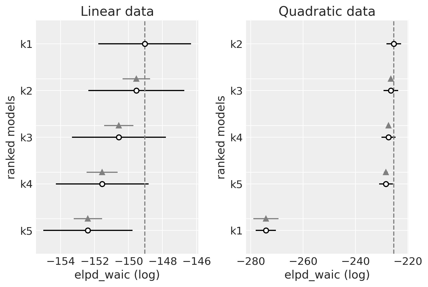
../_images/f6c00036b8abc074007845b4cfde73eeaa3d81a04d2ea53c8b248c5c7d397699.png

观察

我们应该更喜欢具有更高 WAIC 的模型
线性生成的数据（左侧）
- WAIC 在模型之间似乎相当平坦
- 对于更简单的模型，WAIC 似乎是最好的（最高的）。
二次生成的数据（右侧）
- WAIC 在模型之间也相当平坦
- 最差的 WAIC 是 k1，它不够灵活，无法正确拟合数据。
- 对于其余模型，WAIC 非常平坦，但最高的是 k2，应该是这样，并且随着阶数的增加而减小。阶数越高，模型的复杂度越高，但拟合优度基本相同。由于复杂度较高的模型会受到惩罚，我们可以看到我们如何最终选择了可以拟合数据的最简单模型的最佳点。

比较留一法交叉验证 [LOO]#

留一法交叉验证或 K 折交叉验证是另一种非常通用的模型选择方法。但是，要实现 K 折交叉验证，我们需要重复划分数据并在每个分区上拟合模型。这可能非常耗时（计算时间大约增加 K 倍）。在这里，我们应用数值方法，使用后验轨迹，如中建议的那样

dfloo_lin = az.compare(idatas_lin, ic="LOO")
dfloo_quad = az.compare(idatas_quad, ic="LOO")

/var/home/fonnesbeck/repos/pymc-examples/.pixi/envs/default/lib/python3.12/site-packages/arviz/stats/stats.py:792: UserWarning: Estimated shape parameter of Pareto distribution is greater than 0.70 for one or more samples. You should consider using a more robust model, this is because importance sampling is less likely to work well if the marginal posterior and LOO posterior are very different. This is more likely to happen with a non-robust model and highly influential observations.
  warnings.warn(
/var/home/fonnesbeck/repos/pymc-examples/.pixi/envs/default/lib/python3.12/site-packages/arviz/stats/stats.py:792: UserWarning: Estimated shape parameter of Pareto distribution is greater than 0.70 for one or more samples. You should consider using a more robust model, this is because importance sampling is less likely to work well if the marginal posterior and LOO posterior are very different. This is more likely to happen with a non-robust model and highly influential observations.
  warnings.warn(
/var/home/fonnesbeck/repos/pymc-examples/.pixi/envs/default/lib/python3.12/site-packages/arviz/stats/stats.py:792: UserWarning: Estimated shape parameter of Pareto distribution is greater than 0.70 for one or more samples. You should consider using a more robust model, this is because importance sampling is less likely to work well if the marginal posterior and LOO posterior are very different. This is more likely to happen with a non-robust model and highly influential observations.
  warnings.warn(
/var/home/fonnesbeck/repos/pymc-examples/.pixi/envs/default/lib/python3.12/site-packages/arviz/stats/stats.py:792: UserWarning: Estimated shape parameter of Pareto distribution is greater than 0.70 for one or more samples. You should consider using a more robust model, this is because importance sampling is less likely to work well if the marginal posterior and LOO posterior are very different. This is more likely to happen with a non-robust model and highly influential observations.
  warnings.warn(
/var/home/fonnesbeck/repos/pymc-examples/.pixi/envs/default/lib/python3.12/site-packages/arviz/stats/stats.py:792: UserWarning: Estimated shape parameter of Pareto distribution is greater than 0.70 for one or more samples. You should consider using a more robust model, this is because importance sampling is less likely to work well if the marginal posterior and LOO posterior are very different. This is more likely to happen with a non-robust model and highly influential observations.
  warnings.warn(
/var/home/fonnesbeck/repos/pymc-examples/.pixi/envs/default/lib/python3.12/site-packages/arviz/stats/stats.py:792: UserWarning: Estimated shape parameter of Pareto distribution is greater than 0.70 for one or more samples. You should consider using a more robust model, this is because importance sampling is less likely to work well if the marginal posterior and LOO posterior are very different. This is more likely to happen with a non-robust model and highly influential observations.
  warnings.warn(

dfloo_lin

	rank	elpd_loo	p_loo	elpd_diff	weight	se	dse	warning	scale
k1	0	-149.078077	2.346511	0.000000	1.0	2.737718	0.000000	False	log
k2	1	-149.628033	3.043065	0.549956	0.0	2.844436	0.810043	False	log
k3	2	-150.801629	3.927352	1.723552	0.0	2.801148	0.847152	True	log
k4	3	-152.029746	4.897199	2.951669	0.0	2.795982	1.007137	True	log
k5	4	-153.012995	5.546289	3.934919	0.0	2.724531	0.966067	True	log

dfloo_quad

	rank	elpd_loo	p_loo	elpd_diff	weight	se	dse	warning	scale
k2	0	-225.425183	3.036133	0.000000	1.000000e+00	2.829775	0.000000	False	log
k3	1	-226.695683	4.045707	1.270500	0.000000e+00	2.830260	0.400133	True	log
k4	2	-227.955108	4.968154	2.529925	0.000000e+00	2.763448	0.935276	True	log
k5	3	-229.115931	5.843808	3.690748	0.000000e+00	2.771985	1.041893	True	log
k1	4	-274.385064	3.495793	48.959881	1.628497e-11	3.977377	4.888616	False	log

_, axs = plt.subplots(1, 2)

ax = axs[0]
az.plot_compare(dfloo_lin, ax=ax, legend=False)
ax.set_title("Linear data")

ax = axs[1]
az.plot_compare(dfloo_quad, ax=ax, legend=False)
ax.set_title("Quadratic data");

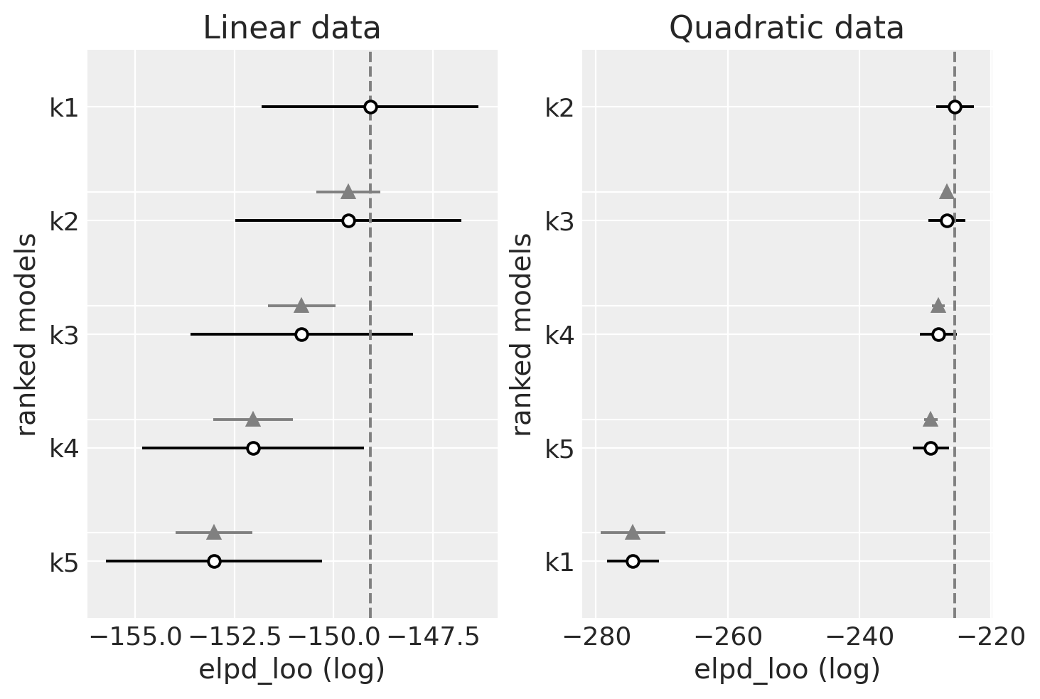
../_images/ed7699a6e25a231bc26bf80eef6c6a66b58388a41e553907dfd9eb8b4d47dadc.png

观察

我们应该更喜欢具有更高 LOO 的模型。您可以看到 LOO 与 WAIC 几乎相同。那是因为 WAIC 与 LOO 在渐近意义上相等。但是，PSIS-LOO 据说在有限情况下（在弱先验或有影响力的观察下）比 WAIC 更稳健。
线性生成的数据（左侧）
- LOO 在模型之间也相当平坦
- LOO 似乎也是最适合（最高）更简单模型的。
二次生成的数据（右侧）
- 与 WAIC 相同的模式

最终评论和提示#

重要的是要记住，随着数据点的增加，真实的底层模型（我们用于生成数据的模型）应该优于其他模型。

一些人认为 PSIS-LOO 提供了模型质量的最佳指示。引用 avehtari 的评论：“我还建议使用 PSIS-LOO 而不是 WAIC，因为它更可靠，并且具有更好的诊断效果，如中讨论的那样，但如果您坚持要使用一个信息准则，那么就留下 WAIC”。

或者，Watanabe 说 “WAIC 是泛化误差的更好近似，而不是 Pareto 平滑重要性抽样交叉验证。Pareto 平滑交叉验证可能是交叉验证的更好近似，而不是 WAIC，但它不是泛化误差的更好近似”。

参考文献#

[1]

Tomohiro Ando。用于评估分层贝叶斯和经验贝叶斯模型的贝叶斯预测信息准则。Biometrika，94(2):443–458, 2007。 doi:10.1093/biomet/asm017。

另请参阅

Thomas Wiecki 对 Cross Validated 上一个问题的详细回复
Aki Vehtari 的交叉验证常见问题解答

作者#

由 Jon Sedar 于 2016 年 1 月创作 (pymc#930)
由 Junpeng Lao 于 2017 年 7 月更新 (pymc#2398)
由 Ravin Kumar 于 2019 年 5 月重新执行 (pymc#3397)
由 Alex Andorra 和 Michael Osthege 于 2020 年 6 月重新执行 (pymc#3955)
由 Raul Maldonado 于 2021 年 3 月更新 (pymc-examples#24)
由 Abhipsha Das 和 Oriol Abril 于 2021 年 6 月更新 (pymc-examples#173)
由 Chris Fonnesbeck 于 2024 年 12 月更新 (pymc-examples#761)

水印#

%load_ext watermark
%watermark -n -u -v -iv -w -p theano,xarray

Last updated: Mon Dec 23 2024

Python implementation: CPython
Python version       : 3.12.5
IPython version      : 8.27.0

theano: not installed
xarray: 2024.7.0

numpy     : 1.26.4
arviz     : 0.19.0
bambi     : 0.15.0
pymc      : 5.19.1
seaborn   : 0.13.2
matplotlib: 3.9.2
pandas    : 2.2.2
ipywidgets: 8.1.5
xarray    : 2024.7.0

Watermark: 2.5.0

许可声明#

本示例库中的所有 Notebook 均根据 MIT 许可证提供，该许可证允许修改和再分发以用于任何用途，前提是保留版权和许可声明。

引用 PyMC 示例#

要引用此 Notebook，请使用 Zenodo 为 pymc-examples 存储库提供的 DOI。

重要提示

许多 Notebook 都改编自其他来源：博客、书籍……在这种情况下，您也应该引用原始来源。

另请记住引用您的代码使用的相关库。

这是一个 bibtex 中的引用模板

@incollection{citekey,
  author    = "<notebook authors, see above>",
  title     = "<notebook title>",
  editor    = "PyMC Team",
  booktitle = "PyMC examples",
  doi       = "10.5281/zenodo.5654871"
}

渲染后可能如下所示

分类

标签